Overview

For our course projects, one was meant to do a project where they try to recreate the results of some circuit, or portion of one, published in a recent paper. Our professor offered a second option which I decided to take, which was porting a statistical simulation for SERDES his lab had created from MATLAB to Python.

Thus my project was adapting and converting their internal statistical simulation system for SERDES systems, initially called StatEye, from MATLAB to Python. It’s primary goal was to estimate the quality of communication in a system based on the resulting bit error rate from all the influences present to aid or impede communication.

The original MATLAB codebase was about 5000 lines. My porting efforts were successful, and along the way I even made a couple of tweaks that were back-ported into the original MATLAB codebase! It is currently going to be used to help teach the next group of students and will eventually be officially released to the public by the lab.

Requirements

The main goal of this project was to maintain functional and performance parity with the MATLAB version I was basing my work on.

• Perform statistical analysis of SERDES links based on Touchstone (.s4p) files
• Output performance metrics
• Have feature to automatically optimize the data link

Objectives

• Match the results of the MATLAB to within 5%
• Match or shorten the execution time of simulations

Takeaways

• Porting to Python from MATLAB was either super trivial, or super difficult depending on the portion of code.
• When porting a program, work backwards from the output to the input. This way one can verify their work on earlier sections and isolate issues more quickly with a reliable output [plotting] stage than without.

Background

In “Integrated Circuits for Digital Communications”, ECE1392, we learned about the fundamentals of Serializer and Deserializers that form the backbone of modern high speed communications. These SerDes (also SERDES) were a mix of analog and digital circuitry and for our class we had to complete individual projects.

In the class we had to each do an individual project that would span the entire semester. In general these were design projects where one would need to find a SERDES circuit they found interesting in a recent paper and then recreate some portion of it and simulate it. I however, took an alternative project.

The professor teaching the class had us use a collection of scripts written by his group in MATLAB to learn and observe the basics of different SERDES concepts. He was interested in having the code converted over to Python so they would be more accessible to the greater research community. I decided to take this as my project to get more familiar with the general theory of SERDES and also strengthen my Python skills.

SERDES Basics

Serializers and deserializer systems are composed of multiple components. At the top level there were three components: the transmitter (serializer), the communication channel, and the receiver (deserializer). There are a few main phenomenon that SERDES tries to contend with through improved designs so that higher communication speeds can be achieved:

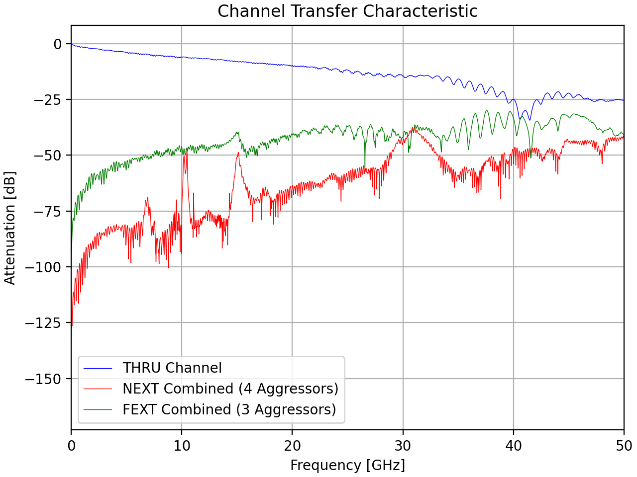
• Channel attenuation - As speeds increase, channels attenuate the signal more from one end to another making them harder to register at the receiver
• Random noise - All electronics are non-ideal and will introduce some degree of noise to the electric signals that pass through them
• Cross talk - Due to the high frequency switching of communications lines, they emit electro-magnetic emissions that influence the state of neighbouring lines, more prevalent at higher frequencies
• Distortions - Again due to non-ideal components, they will have non-ideal (non-linear) responses
• Jitter - Although communications happen at a stable frequency generally, the exact timing of each cycle may not be exactly the same so sampling points may not be at the optimum time
• Inter-symbol interference (ISI) - based on the levels the transmission line was held at and the ones that follow, a given symbol may not be at the expected ideal level. E.g. a single high in a string of lows may not be as evident of a high compared to a string of successive highs.

The path information takes in our generalized model is:

1. Encoding - Converting binary data into symbols for transfer
2. Pre-Emphasis - Adjust the exact output levels based on the symbols that have just been sent and those soon to be sent in addition to the current symbol to try and minimize ISI
3. Digital to Analog Conversion - Driving the output of the transmitter to the desired level
4. Transmission - Data passing through the channel
5. Amplification - Receiver amplifies the incoming signal
6. CTLE - Continuous Time Linear Equalization, an amplification/filtering stage designed to compensate for channel attenuation
7. Analog to Digital Conversion - Sample the channel for digital processes that follow
8. FFE - Feed Forward Equalizer, generate a weighted sum of the symbols adjacent to the main symbol to compensate for ISI
9. DFE - Decision Feedback Equalizer, adjust the output of the FFE based on the previous few decoded symbols and a weighing scheme, also intended to reduce ISI
10. Slicer - Decode the “analog” symbol value to a digital one based on some thresholds

There is more to cutting edge SERDES design but this was the focus of our class and it aligns with what StatOpt simulates.

All in all, the object of SERDES design is to design a system so that data is communicated reliably through the channel with a low error rate. This metric: Bit Error Rate (BER), is the measure of how frequently our receiver decodes a symbol incorrectly. It is generally expressed as a portion of data which is erroneously decoded, e.g. “2.4*10^-5” if 24 in 1 000 000 bits are received wrong. Thus a lower BER is what is sought in designs.

Operation of StatOpt

StatOpt is a statistical simulation of a SERDES system. So instead of simulating the behaviour of the system by running a simulation in the time domain, all influences are modelled as probability distributions which are then combined. This is generally a quicker a more direct way to get the probability distributions one needs to estimate the performance of a SERDES system.

In addition to the statistical simulation, StatOpt also offers the ability to optimize a SERDES system by adjusting user desired parameters, hence the name StatOpt.

User Operation

StatOpt is meant to be relatively straight forward for users to employ. The user configured the simulation by listing their desired parameters in a a file (there were some examples) and upload any desired channel description files prior to running the main script. To quote the full setup procedure from the readme:

1. Upload desired Touchstone (.s4p) files and/or .mat files to describe distortion or pulses.
   • Files for channels need to go into the /channels/ folder. (Both .s4p and .mat channel descriptions).
   • All others (predefined pulses, distortion, etc.) are to be kept in the base directory, alongside this readme file.
2. Configure simulation settings to match desired parameters. Check the example files for baseline configurations.
   • Refer to desired files for channels
   • Set desired output plots
   • Adjust the amount of taps in equalizers
   • Select the parameters to be adjusted in the adaption process, if enabled
3. Adjust the statopt.py script to read the simulation configuration function from the desired simulation file.
4. Run the statopt.py script.
   • If the simulation is expected to take a long time, the user will need to confirm that they want the simulation to proceed.
5. Wait for the simulation to complete.
6. Enjoy the results!

Internal Operation

The internal operation of StatOpt can be broken into four main parts which are executed in the following order:

1. Configuration - Reading in and parsing the user configuration parameters such as communication frequency
2. Simulation - Performing the actual system simulation
3. Adaption - Perform genetic optimization algorithm on system (if requested in configuration)
4. Outputting Results - Primarily through visual plots, although some key metrics are printed to the terminal such as BER

If adaption is enable then parts 2 and 3 are repeated until the optimization algorithm is satisfied.

User Configuration

The first step is to read in the user’s simulation parameters (also called “knobs”) from their configuration file. This is a function generateSettings() which just returns a simulationSettings object with all the fields populated as desired. Given the number of settings available, they are grouped by the segment of StatOpt they affect like the receiver characteristics or adaption process. Below is an example of some sections in a typical generateSettings() function.

# Frequency
simSettings.general.symbolRate.value = 32e9 # symbol rate [S/s] (or 2x frequency [Hz])
    
# Signaling mode ('standard','1+D','1+0.5D','clock')
simSettings.general.signalingMode = 'standard'

... # Other settings

# Impulse cursor length
simSettings.transmitter.preCursorCount.value = 2 
simSettings.transmitter.postCursorCount.value = 4

# Pre-emphasis
simSettings.transmitter.EQ.addEqualization = True

... # Other settings

# Make cross-talk channels asynchronous
simSettings.channel.makeAsynchronous = True

# Channel file names (ensure channel data has same frequency points)
simSettings.channel.fileNames.thru = 'C2M__Z100_IL14_WC_BOR_H_L_H_THRU.s4p'
simSettings.channel.fileNames.next1 = 'C2M__Z100_IL14_WC_BOR_H_L_H_NEXT1.s4p'
simSettings.channel.fileNames.next2 = 'C2M__Z100_IL14_WC_BOR_H_L_H_NEXT2.s4p'
simSettings.channel.fileNames.next3 = 'C2M__Z100_IL14_WC_BOR_H_L_H_NEXT3.s4p'
simSettings.channel.fileNames.next4 = 'C2M__Z100_IL14_WC_BOR_H_L_H_NEXT4.s4p'
simSettings.channel.fileNames.fext1 = 'C2M__Z100_IL14_WC_BOR_H_L_H_FEXT1.s4p'
simSettings.channel.fileNames.fext2 = 'C2M__Z100_IL14_WC_BOR_H_L_H_FEXT2.s4p'
simSettings.channel.fileNames.fext3 = 'C2M__Z100_IL14_WC_BOR_H_L_H_FEXT3.s4p'

... # Other settings

# Noise
simSettings.receiver.noise.addNoise = True
simSettings.receiver.noise.stdDeviation.value = 1e-3 # RX random noise standard diviation [V]
simSettings.receiver.noise.amplitude.value = 0    # RX deterministic noise amplitude [V]
simSettings.receiver.noise.frequency.value = 1e6  # RX deterministic noise frequency [Hz]

Most of the 70 or so knobs need to be populated and given the number of them, users are encouraged to create separate configuration files and direct the main script to read the one they current want to use instead of repeatedly altering a single file. Given the variation in SERDES links that one might simulate, StatOpt has to be able to handle varying sizes to some of the settings like the number of taps in an equalizer or the number of cross talk channels.

Once the user parameters are passed in, parameters that are derived from the user parameters are automatically generated by StatOpt and appended to the settings object. For example determining periods from specified frequencies, or the number of data levels based on the modulation and encoding scheme.

Following a read in of all the parameters, limits are applied to, and then checked against some settings like signal amplitude. These limits are generally the same between simulations and are there to ensure that StatOpt works and returns reasonable results rather than limit what users can do. Should any limits be exceeded then the user is informed and the simulation is stopped.

If all settings are in order, the script continues to simulation.

Simulation

Oh boy, this will be a lot.

Simulation being the primary function of StatOpt, thus it was most of the code. To make the program easier to follow and maintain it was broken into a few segments, loosely following the simplified SERDES component list mentioned in the basics internally for each stage of simulation.

Determining Influences

Given that several hundred simulations could be run during an adaption run some effort was put into streaming the simulations to avoid redundant computations. So there were the “fixed” and “variable” influences on the SERDES link. Fixed influences are not influenced by the “design” of the link, like channel behaviour, and thus are only calculated and summarized once at the start of the simulation. Variable influences on the other hand need to be recalculated for different design parameters like equalizer weights, so these were part of the adaption loop.

Pulse Generation

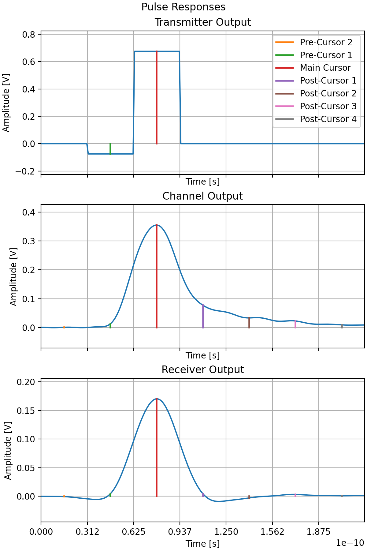
Once all influences are determined, they are then applied to a pulse to find the system’s pulse output when transmitted, the signal received at the other end of the channel, and the final output when processed by the receiver. These pulses will be used in the next stages. For simulations with crosstalk, pulse responses are also generated for each of the aggressor channels.

The length of the pulse response recorded is the same as the number of symbols that we need to consider for ISI. So if two pre-cursors, and four post-cursors are to be considered, then the pulse recorded will be seven symbols long, with the pulse (main cursor) located in the third symbol.

Inter-Symbol Interference

The first step in this is determining all the ISI is determining all the series of symbols that are possible given a modulation scheme for the number of pre- and post-cursors the user is interested in considering in their simulation. These are then grouped based on the pre-main-post cursor combinations (the “trajectory”). E.g. in a binary system with two pre- and two post-cursors, 01101 and 11100 are both grouped into the same trajectory of 110.

Once all the combinations have been classified into the trajectories the ISI is determined. This is done by splitting the pulse response into each symbol’s component (i.e. the first portion is the second pre-symbol) and then going through each combination of symbols scaling pulse parts by data levels.

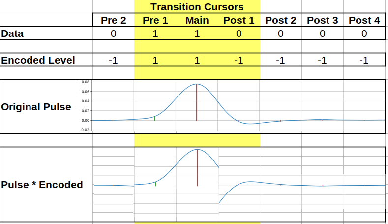
Then for each combination these symbols are then summed together to form the final ISI trajectory for that symbol. When this is done for all combinations the result is a realistic basis of an eye-diagram!

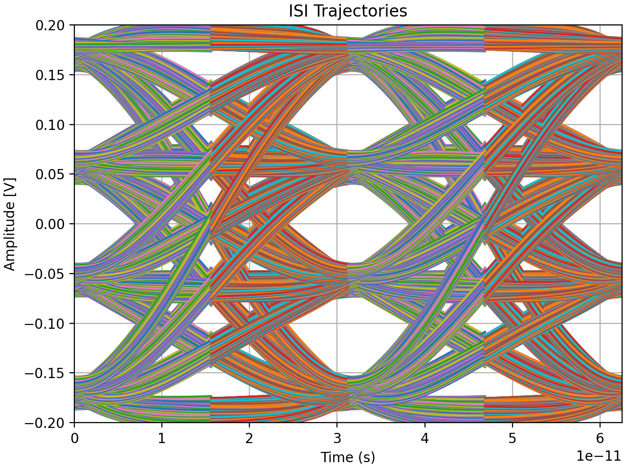
There are some sharp transitions in many of these but that’s an unfortunate result of the operations performed. Fortunately it generally gets smoothed over in the steps that follow.

Generating Probability Distribution

Generating the probability distribution uses the nature of distributions to combine different factors into one overall result using convolutions, both in the time and voltage domain. The process starts by modelling the ISI as a distribution.

The ISI data for each symbol combination for a trajectory is combined and summarized into a distribution for said trajectory. This is repeated for each of the channels in the simulation and stored by channel. The next step is to have cross-talk applied if desired.

Crosstalk is modelled by having all the trajectories for each of the aggressor channels combined into one overall distribution for the channel’s crosstalk influence on the main channel. This summary of the aggressor is convolved to the distribution of the each of the main channel’s trajectories individually.

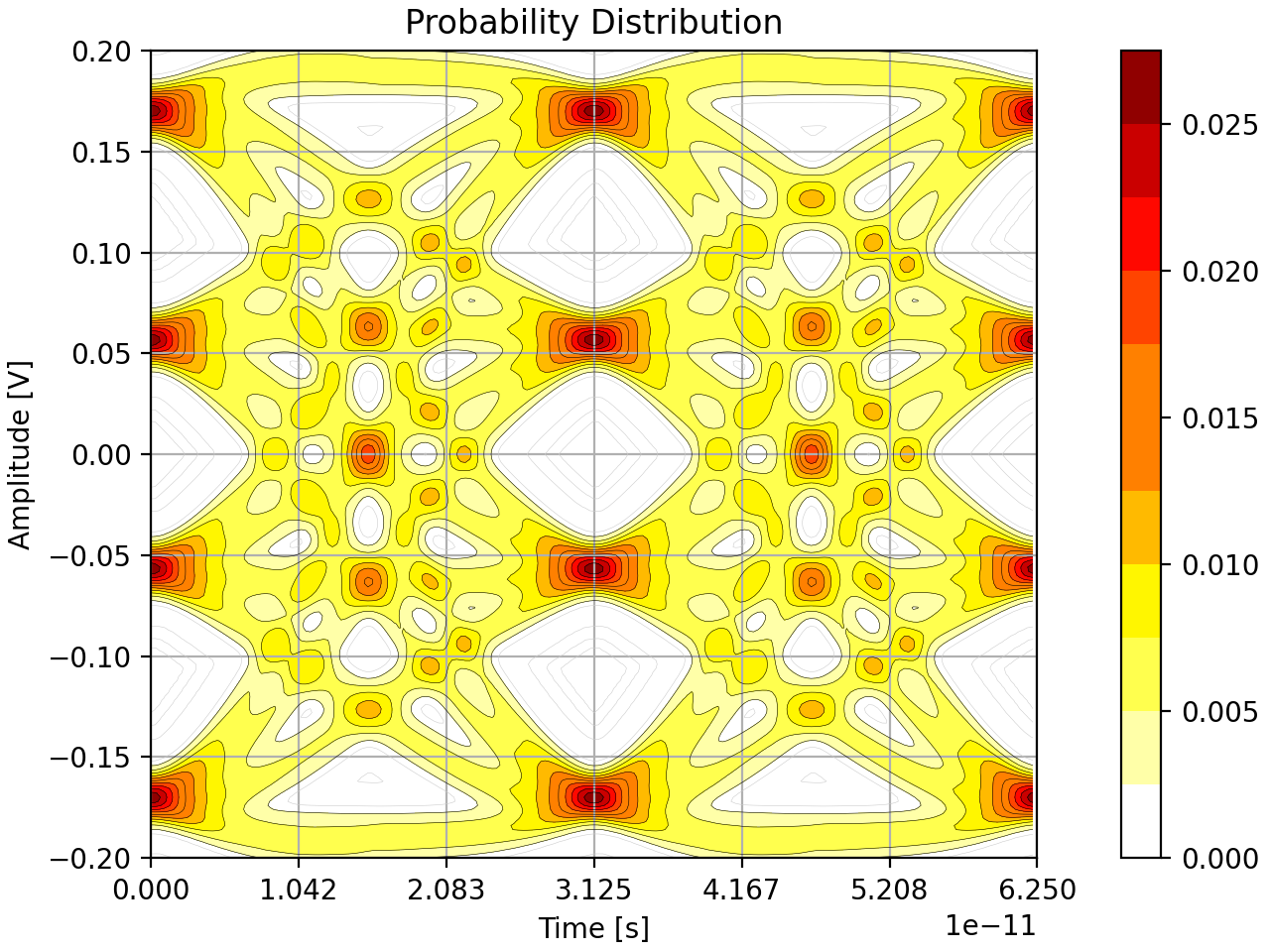
Once crosstalk is applied there is a step to distort the distribution with respect to the distortion described for the transmitter and receiver if enabled. Afterwards two more distributions are applied to the system: a jitter distribution for the receiver and transmitter is used to adjust the distribution in the time domain, and noise distribution to adjust the voltage domain.

After all these operations the final probability distribution is ready for analysis like the figure below. This is the last step that manipulates and generates new data for the simulation of the eye diagram. The remaining steps are focused on processing the data from this step.

Generate BER Distribution

The major analysis performed for each simulation run is determining the system’s bit error rate and how its distributed.

To determine the bit error rate distribution a number of virtual samplers are set on the simulated distribution of their corresponding main cursor levels, e.g. for PAM-4 a sampler for level 2 is used to check all the combinations with 2 as the main cursor. These samplers are used to determine the probability that the signal falls outside the bounds of what that sampler would consider to be the true intended value. Essentially creating bands of BER for each respective sampler. These are then combined to create an overall impression of the BER distribution.

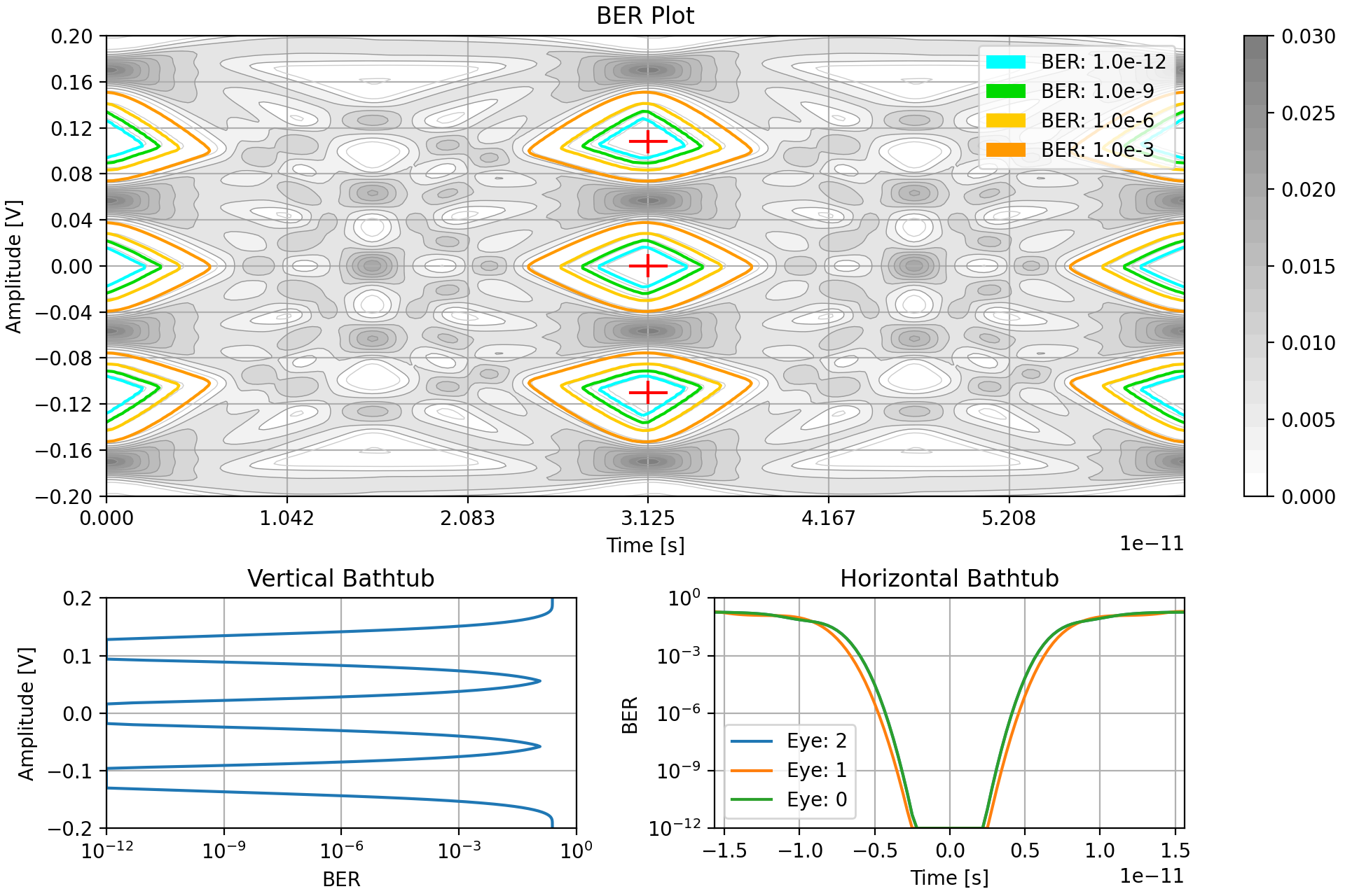
This BER is then analyzed to determine the locations of each eye center and then the “bathtubs” which summarize the BER along the primary axes of the eyes. All these results can then be combined and partially overlaid with the probability distribution for a graphical summary like so.

Analyzing Simulation Results

With all the simulation steps complete, the resulting BER is measured for key characteristics, mainly related to the eye opening(s). These are then recorded to the results object for the simulation run.

• Data levels for the different symbols
• Eye height and width
• Channel operating margin

Adaption

Adaption is an optional feature one can use in StatOpt. With it enabled, the user can select certain design “knobs” (as opposed to any knob, like noise density) for the program to adjust to improve the performance of the the SERDES system. Any collection of knobs can be selected for this purpose, but the usual ones are different equalizer tap weights.

The adaption algorithm is a genetic algorithm, where “generations” are created by deviating from their “parents” on the knobs of interest by some random amount. Each “child” in the generation is simulated, the best best performing ones in a “generation” are used as “parents” for the next generation. There are two stages of adaption: the first stage is a rough search where greater deviations are allowed for the children from their parents so the solution space can be quickly explored. Then there is a fine search where the deviations are limited to a narrower range to try and zero in on the optimal solution.

To avoid redundant simulations, a list of all previously attempted configurations is maintained and checked with each newly generated child.

Outputting

Outputting the data is pretty simple. All of the data used and generated in the simulations is summarized graphically in plots, which are selectively enabled or disabled by the user as part of their simulation configuration. These plots are generally quite simple line or distribution plots.

The most complicated plot is the Bit Error Rate summary plot, which combines a few plots to act as an overall summary of the SERDES link performance. It shows the probability distribution with annotations for different BER frequency regions, and then bathtub plots of the SERDES resilience to jitter and noise.

In addition to the plots, the key characteristics are output to the terminal: data levels for different values, ideal sampling locations, “eye” openings, and channel operating margin for the target BER. Finally, the run time for the script is also printed.

----------Data Level Results----------
Data level 3:  0.170V
Data level 2:  0.056V
Data level 1: -0.056V
Data level 0: -0.170V

----------Sampler Location Results----------
Sampler 2: level:  0.108V, phase:  0.0deg
Sampler 1: level:  0.000V, phase:  0.0deg
Sampler 0: level: -0.110V, phase:  0.0deg

----------Opening Results----------
Eye 0 height: 0.060V, width: 0.28UI for BER: 1.0e-06
Eye 1 height: 0.062V, width: 0.31UI for BER: 1.0e-06
Eye 2 height: 0.060V, width: 0.28UI for BER: 1.0e-06

----------Channel Operating Margin----------
COM: 6.5dB for BER: 1.0e-06

----------Simulation Complete----------
9.661 seconds elapsed since starting the script:
           0.000 to load in and verify simulation parameters
           1.699 to prepare fixed system influences
           6.643 to run simulation and adaption
           1.318 to output data

Porting

I ported code in the order it was executed in the original scripts. The reason being that I believed it would be easier to for me to develop the system incrementally and check my results at each stage to remove any errors before progressing to another portion.

Two things that was consistent across all sections when porting was that I had to accommodate that Python and MATLAB access data: Python uses zero-indexing compared to MATLAB which is one-indexed, and their differences in navigating object fields, which is needed every time settings or the results objects were accessed.

In addition to this, I had to pay attention to Python passing objects by reference rather than by value. So I had to adjust many functions to avoid using the results and settings objects for storing temporary values, or returning and storing the update objects in the main script.

Porting the User Configuration

User configuration porting was pretty simple. I learned and exercised Python concepts about object building and made use of pre-defined classes for certain components like equalizers or noise parameter classes. Given that Python and MATLAB have similar syntax for hardcoding objects and their attributes, the settings functions used as examples needed almost no effort to transition!

The functions that followed to set limits and check them were also largely straightforward to port as well. There was only some minor issues regarding the comparison of divided values since it seems that MATLAB accepts very minute differences in value (due to floating point representation) while Python does not so I manually added a slight margin of acceptable deviation when checking floats for equality.

Porting the Simulation

Porting the simulation was difficult for the initial few stages where the influences needed to be derived since this was where much of the proprietary MATLAB black box library code was employed so I needed to find equivalents in Python.

The first equivalent I depended on was for reading in the channel data from the Touchstone files. For this I used scikit-rf to gather the S-parameter data and then some math to derive the frequency response plot.

Immediately after this, my second major hurdle was to get the pusle response. This originally required the script to approximate the discrete channel response data with a continuous function. In MATLAB there was a function that would provide a rational fit which was then immediately passed into the linear simulation code for pulse responses. I however could not find an equivalent rational fit function or library to use, after some discussion with a friend I followed their suggestion and migrated to the discrete domain instead. This was quite a fundamental change to the way StatOpt functioned but I believe it made the system more accurate in the end and I explain why in that section.

Although my system was now able to calculate realistic and similar pulse responses to the MATLAB, they were not identical so this made testing the code that followed more challenging since they would be acting on different data. To get around this I simply started saving interim results from MATLAB to load into the Python script during development to ensure later stages matched the functionality of the source code.

Luckily the remaining simulation steps used more conventional math related to statistics so I didn’t have too hard a time converting them to use the equivalents offered in NumPy and SciPy.

Porting the Output

Porting the plotting was a pretty simple task, and I should have done it at the start of my efforts so I could use it to graphically compare my progress to the MATLAB from the start. The text output to the console was a quick change in print() calls, so most of my time was spent migrating code to use the matplotlib library for plotting.

Fortunately matplotlib was designed from the ground up to have an almost one to one parity with functions in MATLAB so this wasn’t too difficult. I just had to deal with some of the nuances that differed in their handling of subplots and contour graphs.

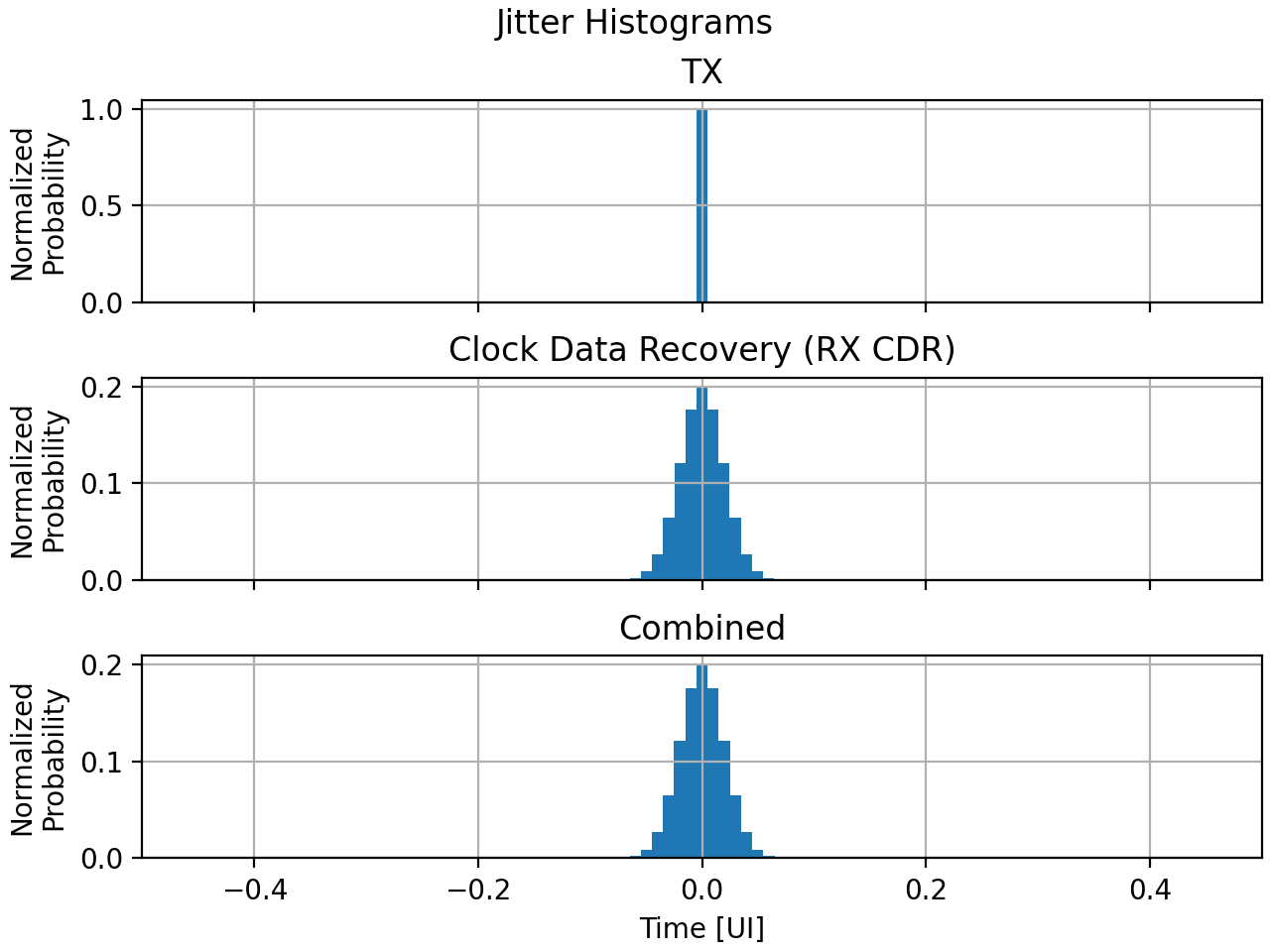
Below is the code used to initialize and prepare the first two plots for jitter in MATLAB. Note that subplot() is called to create and swap between each subplot.

figure('Name','Jitter Distribution');
s(1) = subplot(3,1,1);
bar(TXTime,TXJitter);
title('TX Jitter Histogram');
ylabel('Normalized Probability');
xlabel('Time [UI]');
xlim([-1/2, 1/2]);
grid on;
s(2) = subplot(3,1,2);
bar(RXTime,RXJitter);
title('CDR Jitter Histogram');
ylabel('Normalized Probability');
xlabel('Time [UI]');
xlim([-1/2, 1/2]);
grid on;

Here is the equivalent code in Python where subplots are referred to using axs[x] after making a plot with explicitly 3 subplots.

fig, axs = plt.subplots(nrows=3, ncols=1, sharex='all', dpi=200, num='Jitter Distribution', layout='constrained')
fig.suptitle('Jitter Histograms')
axs[0].hist(TXTime[:-1], TXTime, weights=TXJitter)
axs[0].set_title('TX')
axs[0].set_ylabel('Normalized\nProbability')
axs[0].set_xlim(TXTime[0], TXTime[-1])
axs[0].grid()

axs[1].hist(RXTime[:-1], RXTime, weights=RXJitter)
axs[1].set_title('Clock Data Recovery (RX CDR)')
axs[1].set_ylabel('Normalized\nProbability')
axs[1].grid()

Adaption

With the simulation pipeline in StatOpt completed I worked on implementing adaption since it depended on the rest working correctly first. On its own it was about 20% of the codebase, so working through it took a while until I understood the logic within.

Since this was mostly about making and comparing system configurations, the code didn’t depend on any complicated math, only some random number generation when generating offspring. Most of my time went into adjusting how the system was accessing the data objects so it was in line with the correct methods to do so in Python. In summary the pitfalls I had when working with this beast of object manipulation:

• Accidentally setting the results object to be the returned value of delattr() which is always None
• Improper indexing and enumerating of lists
• Not creating attributes before trying to create their sub-attributes, which is permissible in MATLAB. E.g. With an object A, trying to set A.B.C = 8 without having some value explicitly granted to A.B in advance

Even so, there is one major difference in the port compared to the base MATLAB, the execution time. When running the adaption algorithm in Python it takes between two to three times as long to execute. However for my initial port this was acceptable since the final results were in alignment with MATLAB.

Differences to the Original Version

Although I tried to stay as faithful to the original version of the MATLAB code there were a few places I diverged from the way things originally were. These mostly due to the language or libraries rather than intentional design changes I wanted to enact.

For starters, the figures were not interactive like in MATLAB. This is due to matplotlib generating static plots, so one couldn’t click in a probability distribution for example to see the probability of a given point or the value of a line.

Secondly, I made to make slight adjustments to the way equalizers are handled in the user configuration to make the terminology more consistent across them.

The real difference however was moving the channel modelling from the continuous to discrete domain.

Moving to the Discrete Domain

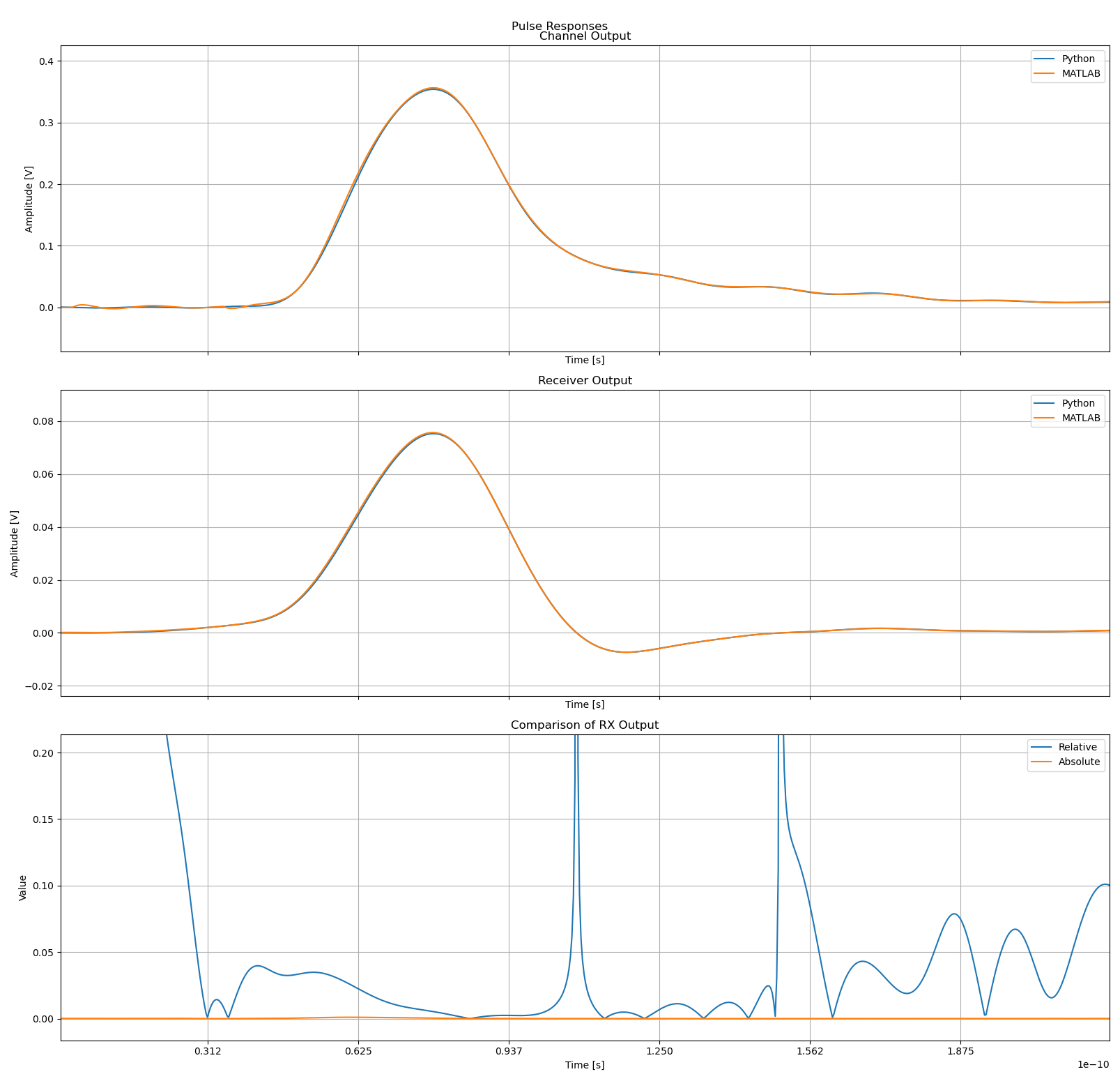
The main divergence I had from the original MATLAB codebase was that I calculated the pulse response using discrete domain math instead of continuous time modelling used in the original scripts. This was originally done due to the lack of an equivalent available to me in Python (and I certainly didn’t have the time to spend trying to code one myself,) however when I was comparing the results I found that the system previously used in MATLAB may have been severely inaccurate!

To recap, in MATLAB the way the pulse response through a channel was simulated was that the channel would be read in as a series of discrete frequency response points. This frequency response would then be fit using a rational polynomial, using the function rationalFit() (in the original version of StatOpt it had 48 terms). This fitted polynomial would then be used as the model of the channel that the pulse would then be subject to using a linear system simulation.

When comparing my results I found that they varied by a fair bit, but was generally under 5% relative deviation for most of the pulse in my tests.

I still wanted to see where this was coming from since I imagined that even though the approaches were different, the source data was identical so the results should have been more in line. So I decided to do a comparison of the fitted curves to the frequency response data they were derived from.

In the plots that follow I group the channels based on the example channel data sets we used for StatOpt examples. The top left plot is always the main channel, and the remaining plots are the crosstalk channels. Orange is the original data, while blue is the fitted function.

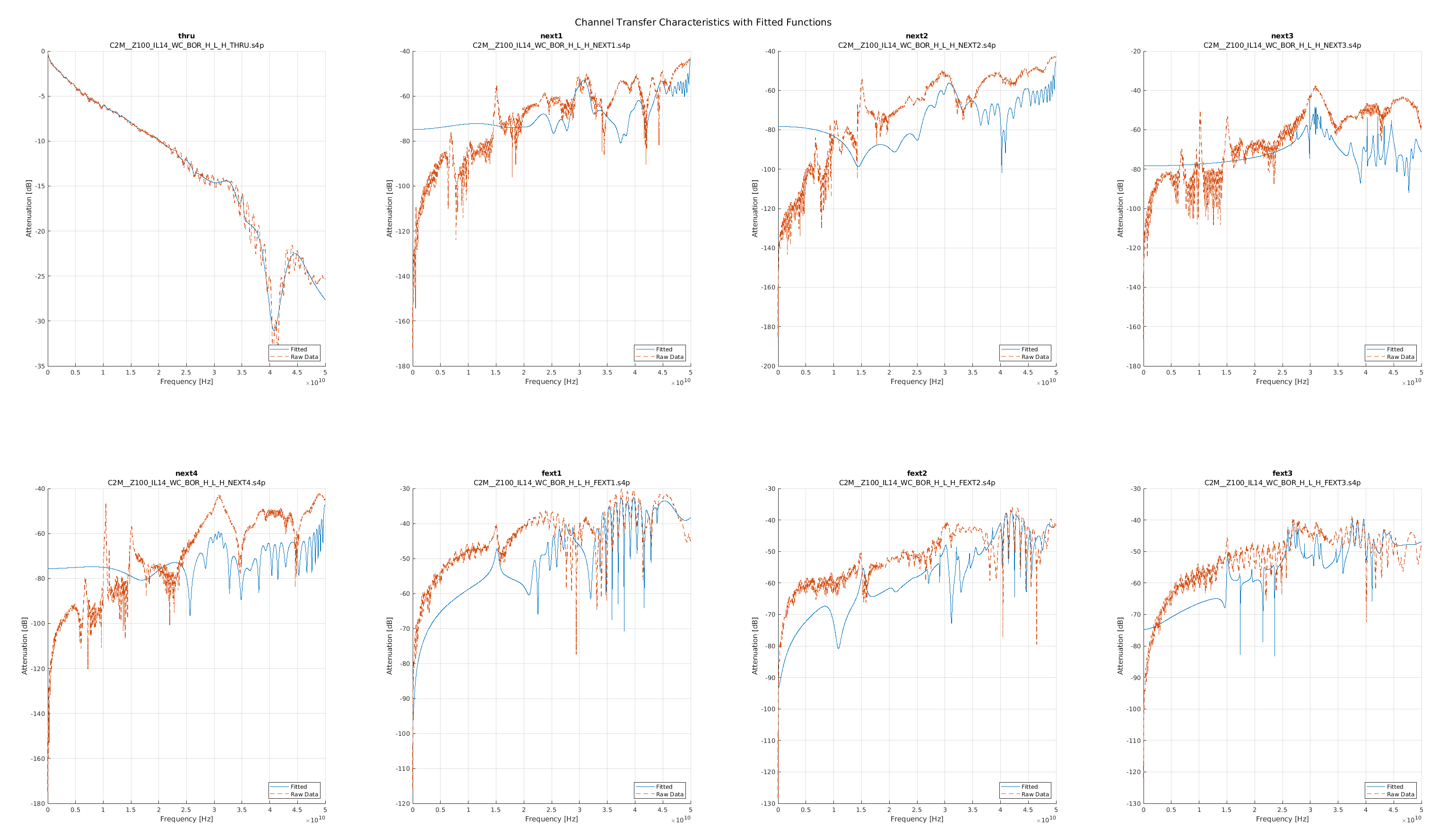
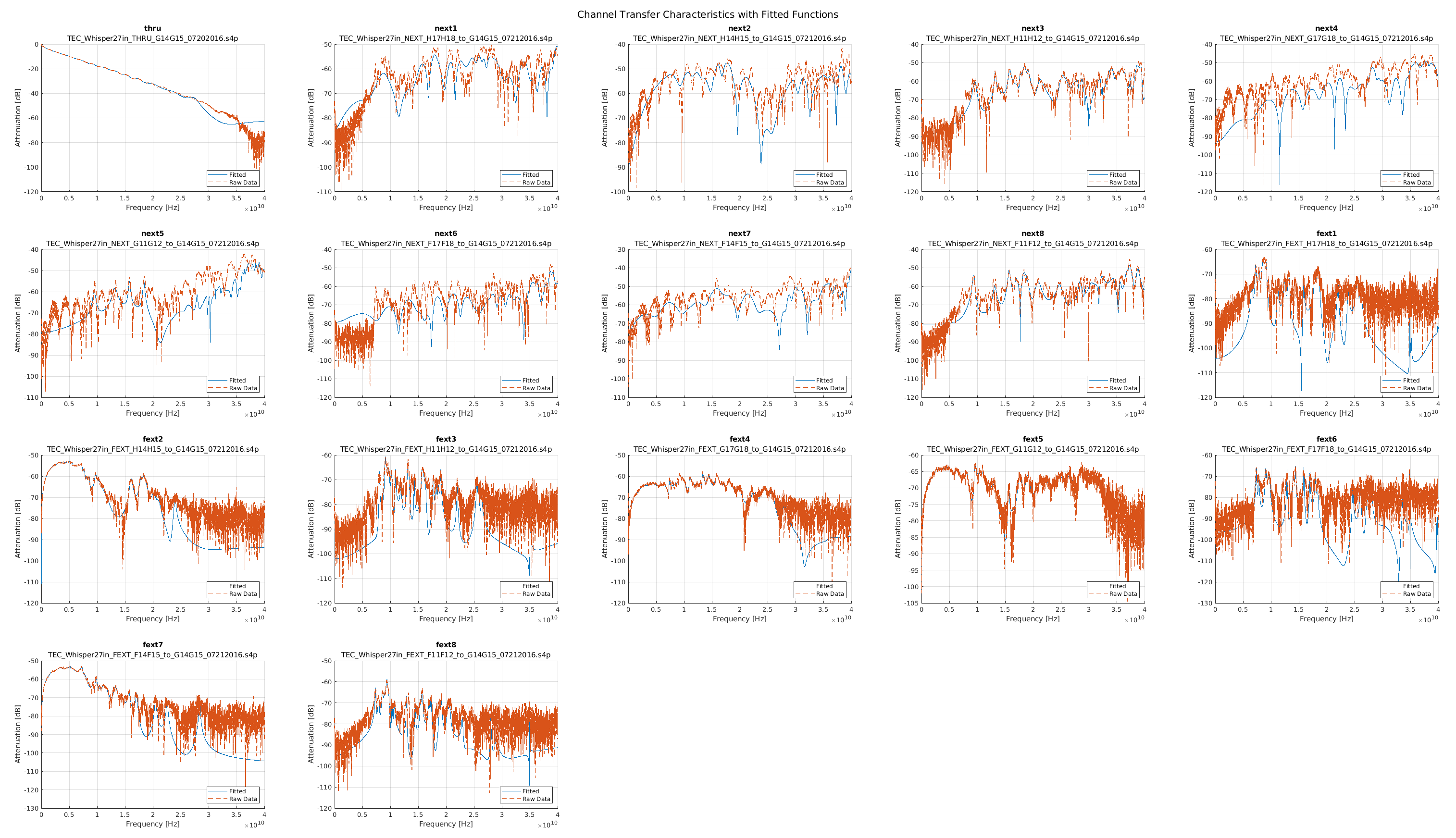
As one can see the fits were not as good as one could hope for the channels, especially for the crosstalk channels. This meant that the linear models used in the MATLAB scripts were not good representations, leading to poor results.

When I showed this to the team they were surprized, but receptive to my critique. The discrete domain approach was accepted as the correct way forward and was actually back-ported into the MATLAB version they now distribute!

Conclusion

StatOpt’s Python port was a success! When compared with the MATLAB version, they both reported the same results once the simulations were all moved entirely to the discrete domain. The only real difference for users was run time.

My professor was pleased with the results I presented in class. In the summer that followed I completed it and helped transition my work back to the lab so they could release it alongside the MATLAB code and also eventually work it into the curriculum for ECE1392 in the form of Jupyter notebooks.

Future Work

The main pain point with the Python port at the present is the run time: the Python version takes almost three times as long to simulate a link, this is especially apparent when performing an optimization run. Doing some profiling on the optimization run time, I found that 90% of the runtime is due to the call to lsim for the CTLE stage to perform linear simulations of the CTLE stage. I suspect this could be reduced by precalculating a convolution to apply in the discrete domain and reusing it instead of calling lsim as had been done for the channel pulse responses.

Other than this rather critical user experience improvement, there are two more improvements I foresee for StatOpt:

• Investigate the use of an alternative, more interactive graphics library for figures like pyqt or Altair
• Consider allowing the chaining of .s4p files to allow systems to be more flexible. For example allowing one to change the transmission line but keeping the same die-to-pad channel.