Overview

For my capstone project in my final year of undergrad I worked with two of my classmates from mechanical engineering on a project for the Advanced Micro and Nanosystems Lab (AMNL) at the University of Toronto. The project was to develop new ways to administer a modern intervention for ischemic strokes which are caused by a blockage in the blood vessels supplying the brain and account for 87% of strokes¹.

Our project was to develop an automated system that would use precisely controlled magnetic fields and an automated feeding mechanism to autonomously guide the guide wire through a network of blood vessels with video feedback (to mimic a CT scan). The goal being to provide a proof of concept for a fully automated EVT system to be used in remote communities where patients would otherwise not have timely access to this procedure.

Our team worked on this until mid January when we had to re-scope to something entirely simulated due to pandemic related measures at the university explicitly prohibiting us from developing physical prototypes.

Our re-scope was to develop a simulation of the wear caused by the guide wire as it is fed through a blood vessel, and use it to develop a path planning method to minimize damage should the tip of the guide wire be controlled as though we were able to complete our initial project.

Although COMSOL Multiphysics was initially considered to make this simulation, we had issues getting it to handle multiple potential collisions due to how we modelled the guide wire, so we instead decided to try and code a simulation from scratch in MATLAB. This was successful, if a bit crude.

My contributions to this project was primarily coding, my teammates worked on reviewing the related literature for guidance and compiling the reports and documents we needed.

Since this project was basically two related but different projects, I will discuss each one separately.

Strokes in Canada

In Canada, strokes are the third leading cause of death¹ and rank tenth in contributing to disability-adjusted life years (a measure of the years lost due to poor health, disability, and premature death)². There are three main types of stroke: ischemic, hemorrhagic, and transient ischemic attack (“mini-stroke”)³. The majority of strokes (87%) are ischemic strokes³, which are caused by the blockage (primarily due to blood clots) of a blood vessel or artery that supplies blood to the brain. When a person suffers from a stroke, neurons begin to die rapidly due to the loss of blood flow. It is estimated that 1.9 million brain cells die each minute during a stroke⁴, meaning urgent treatment is critical to avoid fatality or lasting disability as a result of the stroke.

Acute ischemic strokes are traditionally managed through thrombolysis, the use of medication to break down blood clots⁵. A more recently developed procedure, endovascular thrombectomy (also called mechanical thrombectomy, or EVT), in which the blockage is mechanically removed using a stint carried by a catheter, guided to the location using guide wire. The stent is deployed to capture the blockage before the entire assembly is withdrawn⁵. Patient outcomes when undergoing EVT are significantly improved when compared to treatment through thrombolysis alone⁶. However, only 23 hospitals across Canada could perform EVT⁷ at the time of our project.

The procedure needs to be done rapidly but accurately to ensure a good outcome for the stroke victim. Otherwise it is better to have the victim undergo traditional thrombolysis. As concluded by A. Alawieh, et al.⁸:

“Longer ET procedures lead to lower rates of functional independence and higher rates of sICH and complications. Exceeding 60 min[utes] or 3 attempts should trigger careful assessment of futility and risks of continuing the procedure."

Autonomous Control System

Our project was meant to be about automating the process of navigating blood vessels once the catheter is inserted into the patient, making use of a magnetically influenced guide wire tip.

Current Control System

The catheter for EVT is inserted in the femoral artery, it must then be navigated through various vessels up to the blockage, generally in the skull. This requires the skill and knowledge of a trained surgeon to perform and the specific equipment the manipulate the guide wire accurately.

Accurate navigation of the circulatory system is achieved through the guide wire’s “hooked” end. As it is fed through the blood vessels it can be rotated axially to direct the guide wire through junctions. This gives the system two degrees of control for the operator: rotation of the guide wire, and the amount fed into the patient. Both of these begin to be harder to control as the length of guide wire increases.

The surgeon does not perform this surgery blindly either, a continuous CT or MRI scan is used to help the surgeon know their guide wire’s place in the patient’s body and determine the path to take to the offending blockage.

Our Control System Goal

The system we were aiming to produce would retain some features of the current system. Notably the feedback would be primarily a set of video feeds and the guide wire would still be fed into the vessels using a reel to control the length of guide wire inserted.

The major difference between the typical system and our own was that we would have permanent magnets attached to the tip of the guide wire for the purpose of inducing a force on it in a controlled magnetic field. This would in theory give the user (human or not) navigating the vasculature full control of the tip’s orientation and a limited translational range too. This would raise the degrees of control to essentially all six if executed properly.

One other major change not to the hardware, but to the system overall is the goal to eliminate the need for a human operator. This needed the development of a control algorithm to take their place in both operation planning and execution.

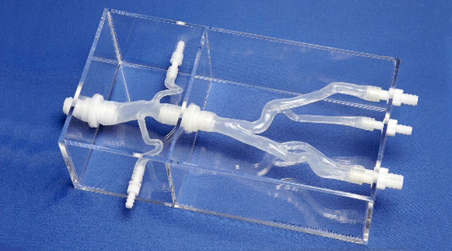
Overall, our goal for the capstone was to have a system capable of taking in a model of the victim’s vasculature, along with a declared start and end point (used for path planning) and then successfully navigate the vessel modelled in reality using video cameras and a “phantom” model in place of an actual blood vessel and CT/MRI scanning.

Requirements

• Use a controlled magnetic field to orient and position the guide wire tip
• Autonomously determine a path through a model between two specified points
• Autonomously execute the path relying solely on visual feedback
• Design or acquire an appropriate guide wire feeding system
• Procedure must not exceed 60 minutes

Objectives

• Minimize tip collisions with vessel walls during navigation
• Maintain position of tip to an accuracy of 0.1mm and 0.1°
• Require only one attempt to navigate the target system

Control System Work

The control system could be broken down into a set of components that had to be developed.

• Vision tracking of the guide wire
• Path planning
• Controlling the hardware (magnetic field generator and reel)
• Control system to ensure positional accuracy

The control system was going to be written in MATLAB. The reasons for this was that it was what we were most familiar with and it had modules that would accelerate the design of certain features, namely vision and control loops. The magnet field generator also had MATLAB examples for how to operate it using MATLAB which would also accelerate our work. By developing it all in MATLAB interfacing our separate code modules would be far smoother than a mixed environment approach.

My primary contributions towards the control system were: path planning and controlling the magnet field generator.

Path Planning

Path planning was composed of two parts: model processing to prepare a map from a 3D model, and then the path finding algorithm itself.

Model Processing

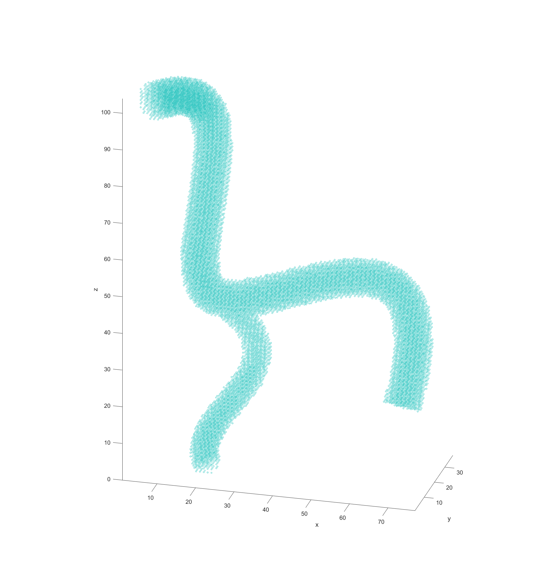
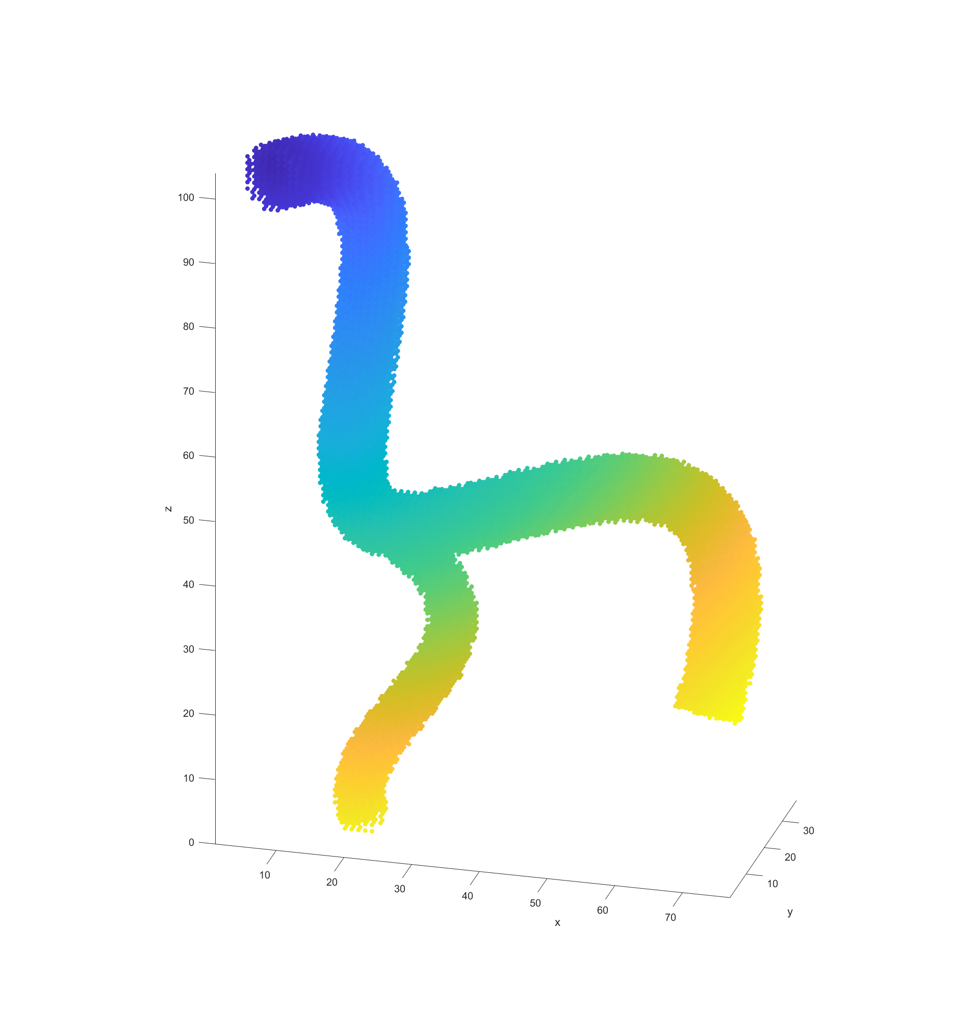
My first task in the project was to determine how we would plan our paths through an arbitrary 3D model. The first thing I settled on was the format we would use as input models, STL files typical of 3D printing. They follow a simple standard that is not proprietary so reading them and converting them into useful data is straightforward, and most 3D software supports outputting STL files as well.

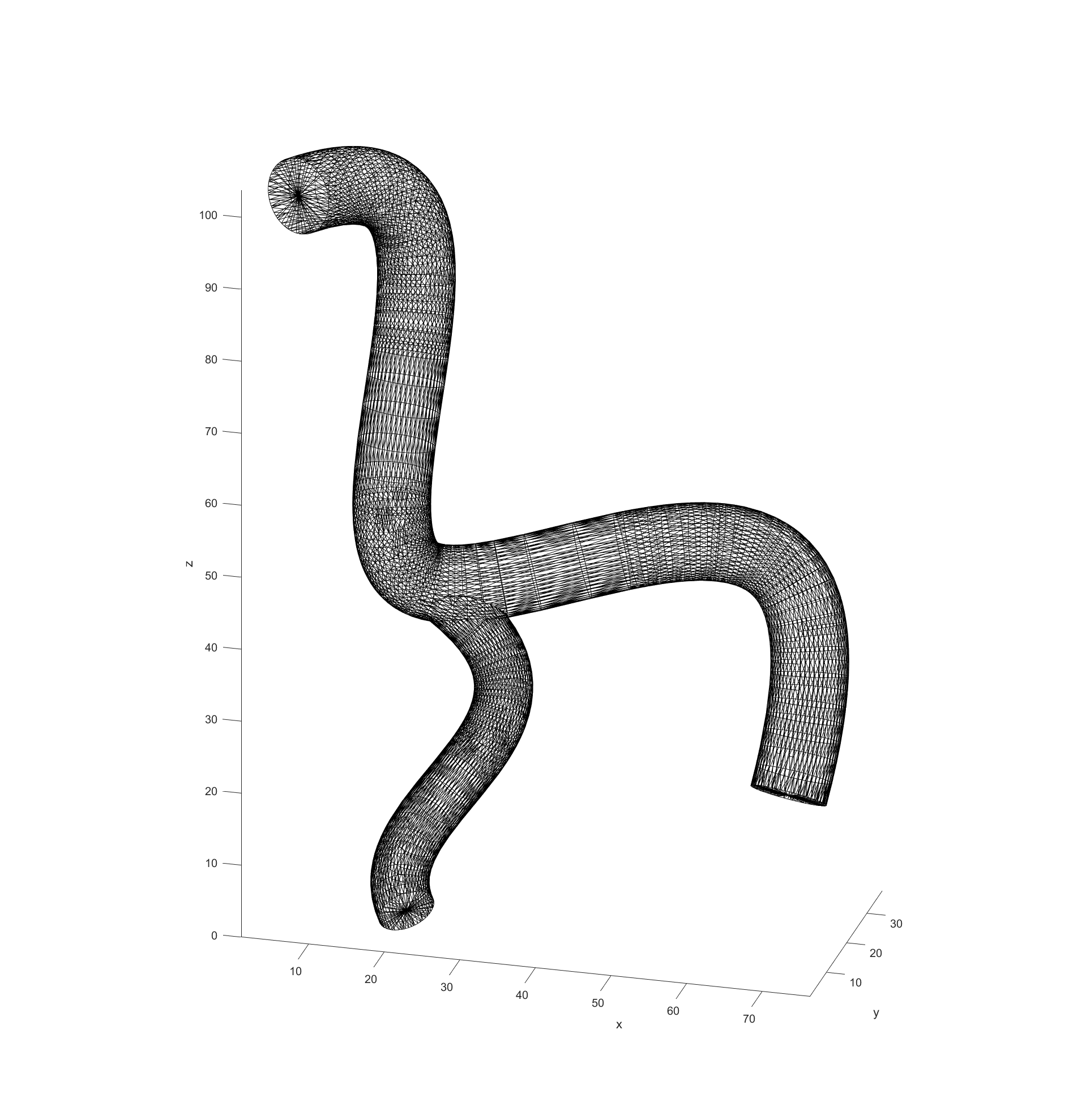
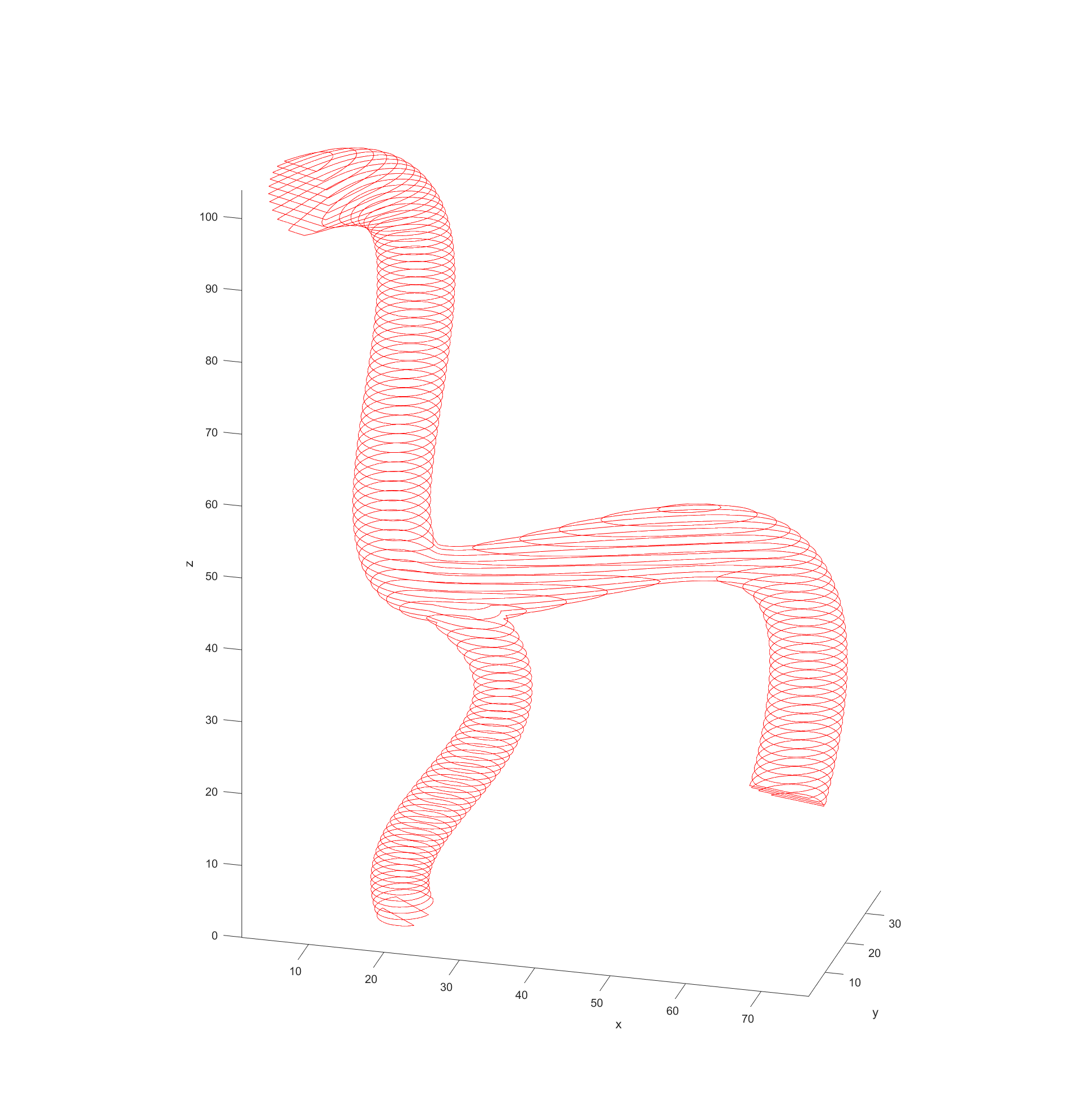
My code would read in the model data from STL files and then turn them into a cloud of nodes to use for navigation in 3D. The first step in this process was to simply see what nodes were valid or not in a regularly spaced 3D grid. This was done by “slicing” the model in regular intervals, which then has a grid of equally spaced points overlaid. Any points that fall within the bounds of the model are marked as valid for path finding. This is repeated for each slice in the model.

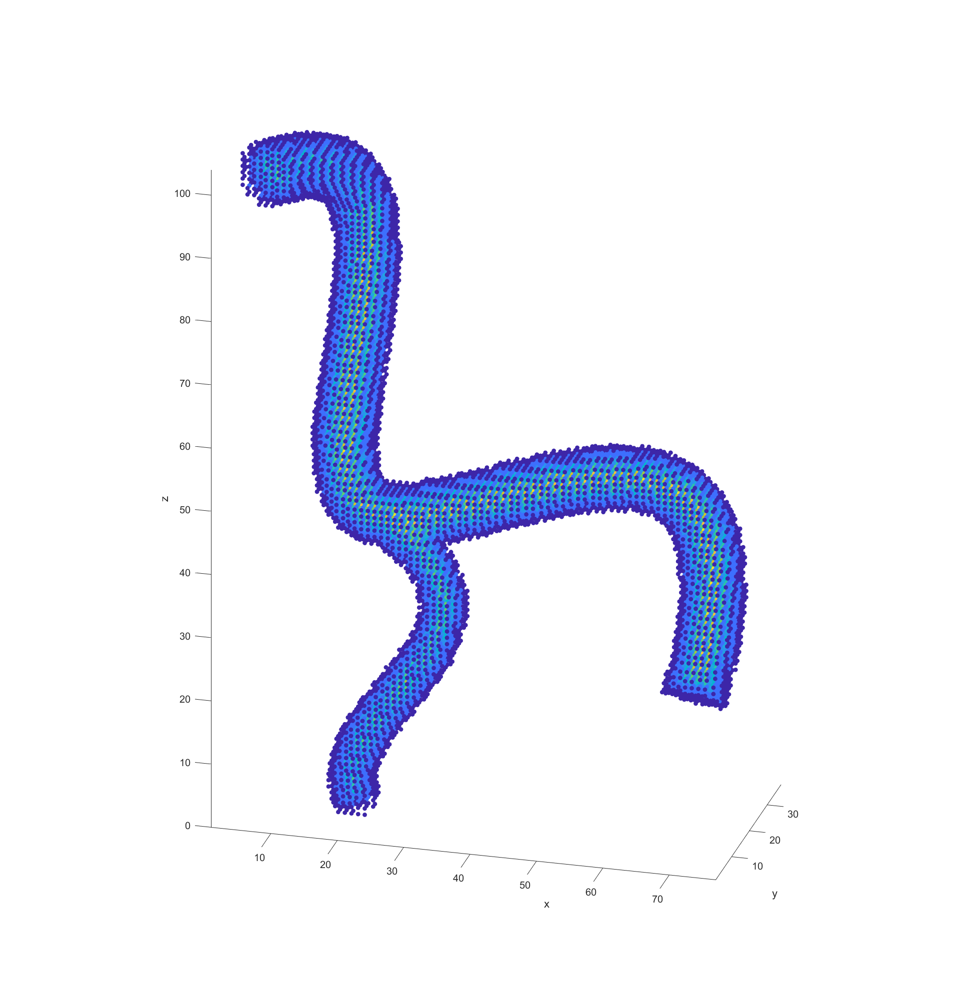
The final step before plotting the path is recording the distance of every valid node to the nearest vessel wall. This was done by initially scanning through all valid nodes if they had a neighbouring node that fell outside of the model (was invalid). These would be marked as “boundary” nodes with a distance of 0 to the vessel wall and a new cycle would begin. This time valid nodes would check for an adjacent boundary nodes and record the distance between themselves and them as its distance to the vessel walls. These cycles would repeat with nodes checking if any neighbours had a distance to the boundary and adding their distance until all valid nodes had a recorded distance.

Path Finding Algorithm

With the processed model and the supplied start and end points, the actual path finding starts by determining the distance between every valid node and the end point and recording it. This step could be argued to be part of model processing but because it is dependant on the path I included it in this section.

With all this data prepared it was time to deploy an algorithm to finally begin plotting a path through the blood vessel as represented by this grid of points. I decided to employ the A* algorithm for path finding because it is computationally efficient and allows the easy addition and weighing of different heuristics, which is vital for this application. For a good path, there are three basic heuristics we considered when selecting nodes:

• Distance to end point
• Distance to vessel walls
• Cumulative distance travelled to the node

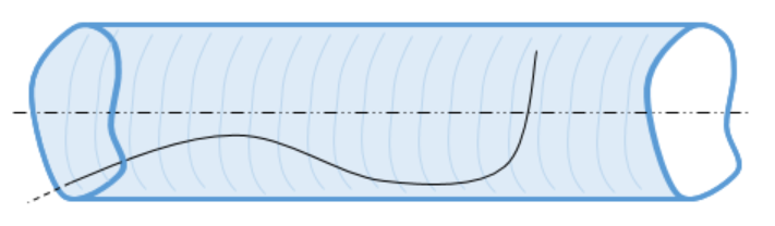
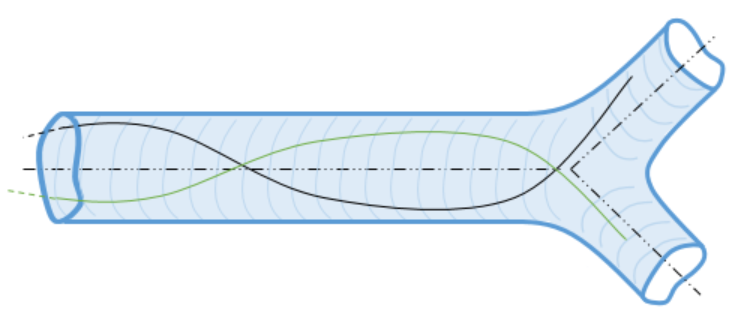
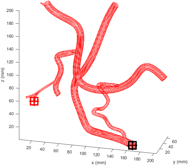
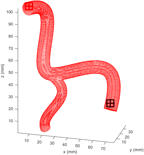
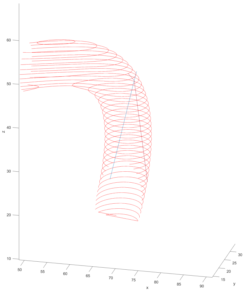
Distance to end point and cumulative distance travelled were both used as “costs” for the path, while distance to vessel walls was treated as a “reward” that would cancel some of the “costs”. The A* algorithm was then used to find the path that would connect the two points with the lowest cost based on these heuristics. In the following examples the path is drawn from the start (black crosshair, bottom right) to the end (red crosshair, left edge), their heuristic weights listed as “distance to end - cumulative travel - distance to vessel walls”.

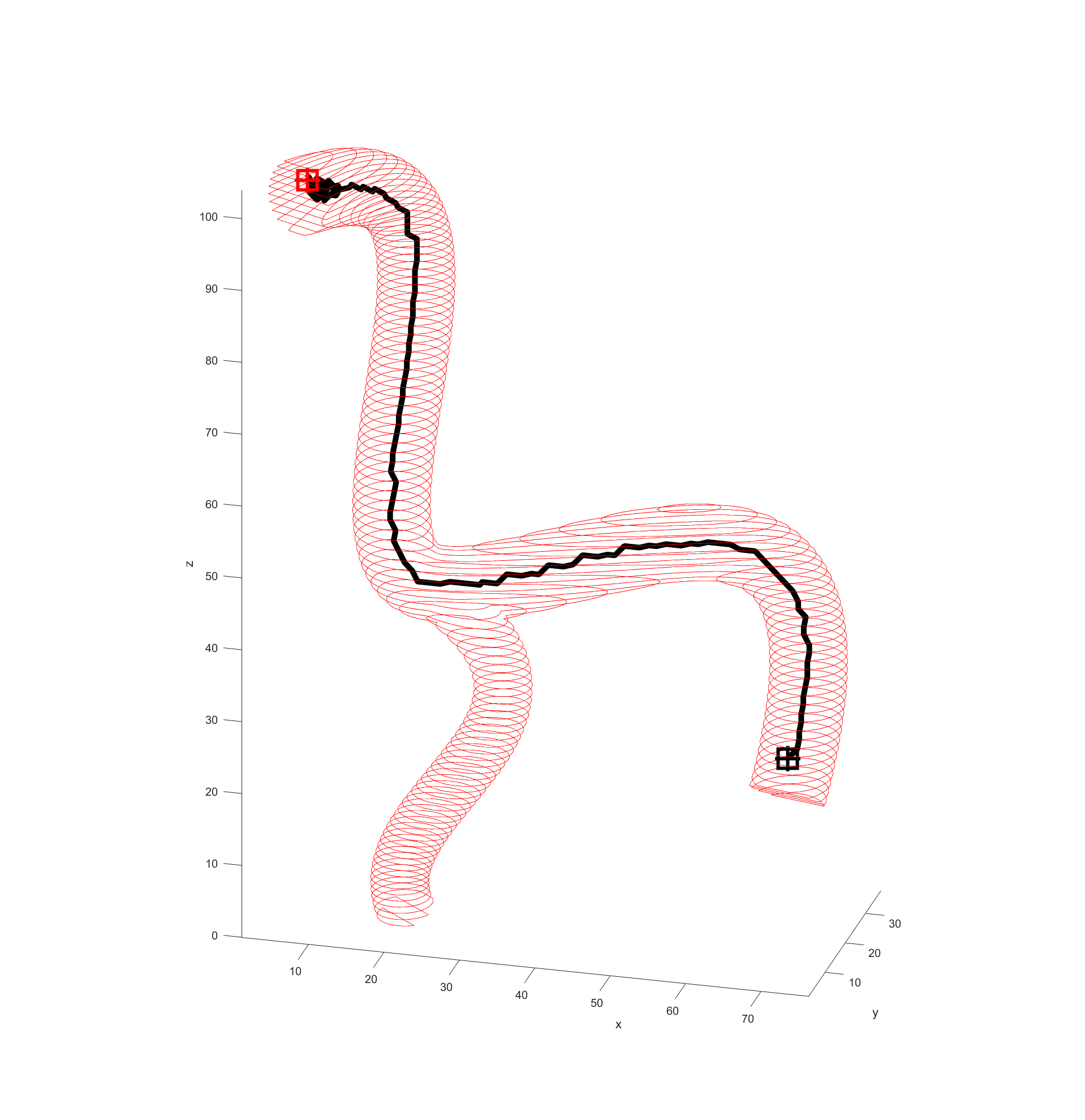
This basic example was enough to prove the system worked but we needed to see how it would handle a more complicated vessel network. Applying the same path finding algorithm to the complicated model we had resulted in this.

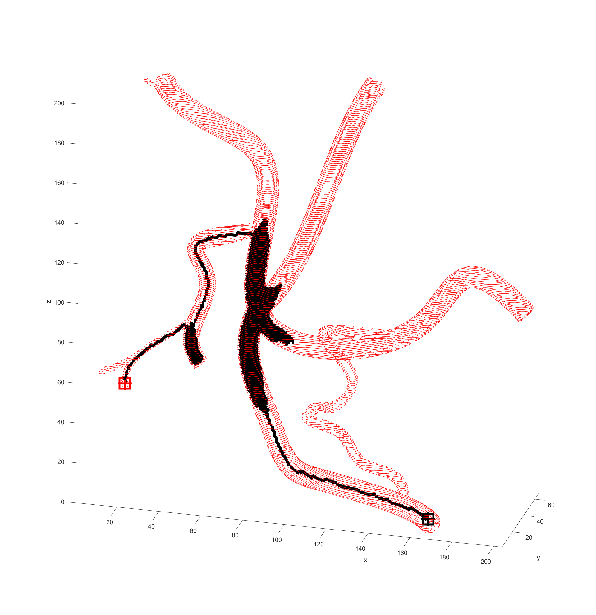
There is significant meandering in the middle where the model partially pulls away from the end point. To see how this could be fixed I wanted to see how each factor affected the results, so I started from a basic equal balance.

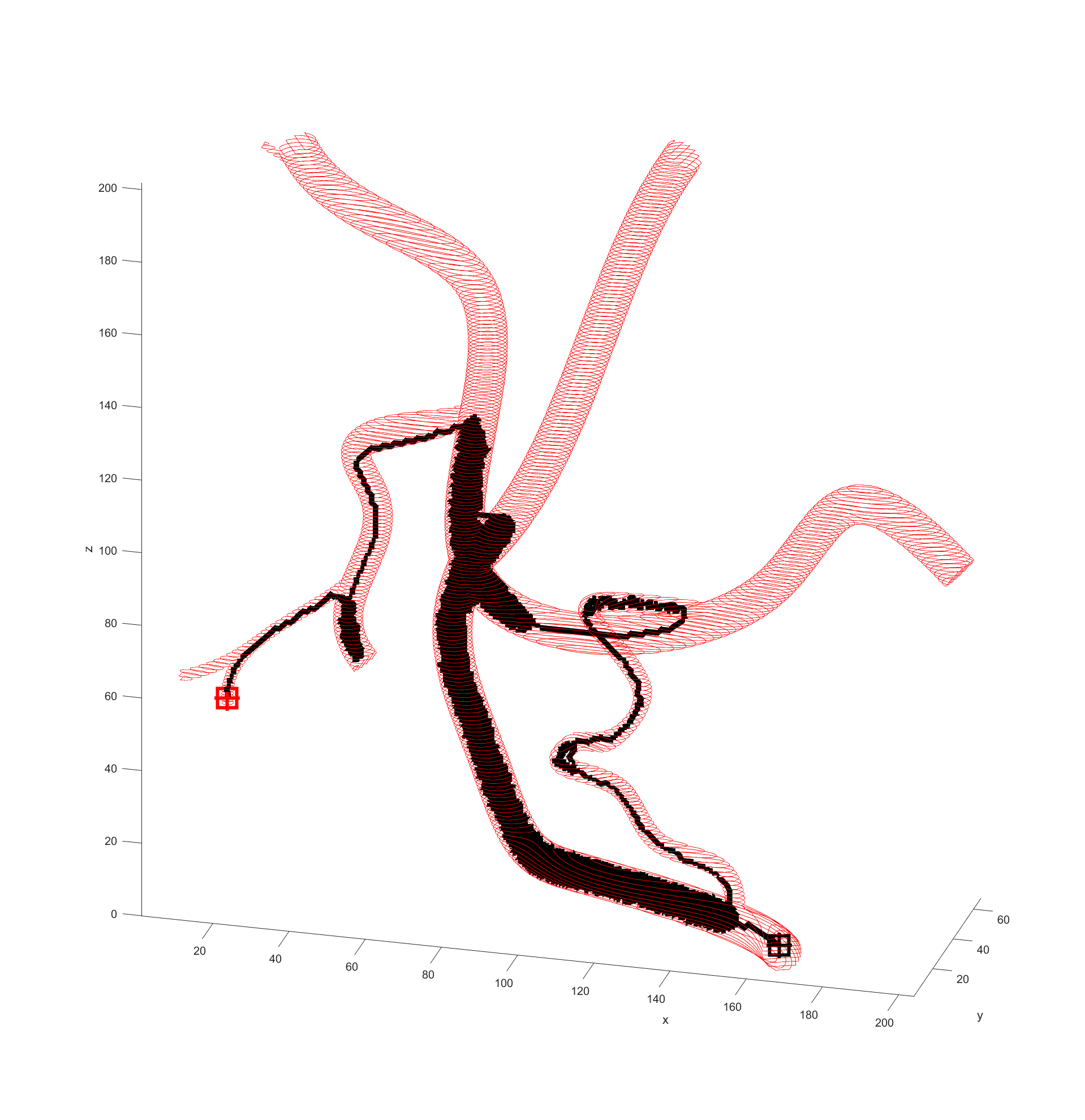
After some more tweaking it was found that increasing the cost of travel prevented this meandering, and keeping the distance to the end point cost equal to the reward for staying away from boundaries prevented the algorithm being hesitant to enter smaller vessels when needed.

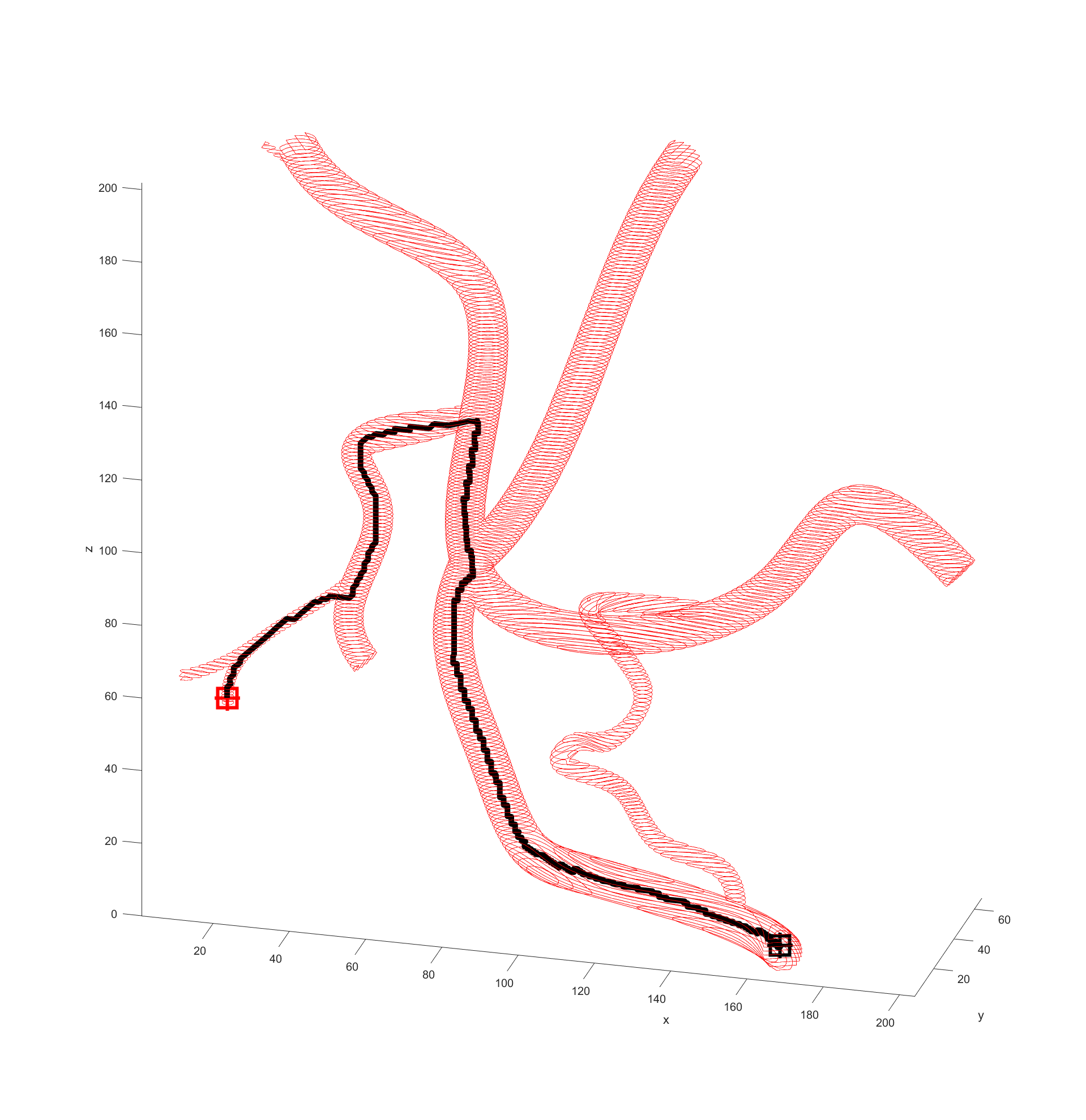
Returning and running this on the simple example revealed a path almost identical to the one previously so this weighting was kept.

I prepared some animations of the paths for presentations and would like to share them here.

Magnetic Field Generation

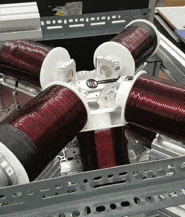
For magnetic field generation we were going to use the lab’s OctoMag magnetic field generator apparatus. This was capable of generating a wide variety of user defined magnetic fields and gradients inside its workspace. It takes care of all the math involved in converting a magnet field to a series of currents in its coils for the user (unless they opt to dictate the currents themselves).

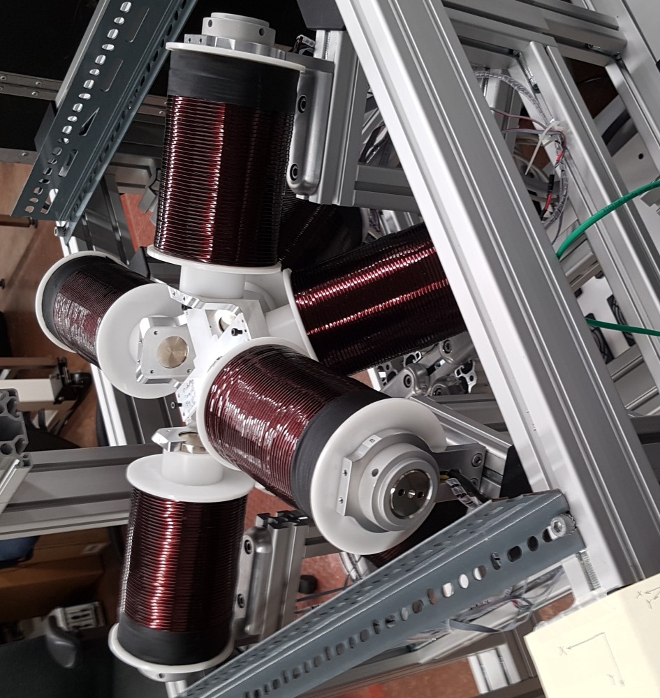
I read through the basic documentation on how to set various fields and gradients as well as imputing some time based functions for fun to get familiar with it. The functions were pretty simple to understand and use like setFieldStrength or setFieldGradient. My experiments led to me spinning a test magnet in the OctoMag.

I stopped there and decided to focus on other course work until the other components were ready and we needed to start “closing” the control loop, namely with vision.

Vision

Vision was handled by a teammate. He worked to enhance the detectability of the small/narrow guide wire in the video feed so we could track it accurately. To process the images he used MATLAB’s image toolkit to apply convolutions to help make out the narrow dark curve of the guide wire in the otherwise largely white image. Further conditioning was needed to determine the state of the tip as this is what our focus was for control.

There was some promising results coming from his images, although it seemed that lighting was the determining factor in whether or not an image would be processed properly or not.

Reel Hardware + Control

The reel hardware was being developed by my other teammate. She was successful in designing some hardware for this, however this came shortly before we were forbidden to make or test using any prototypes by faculty. So we were unable to actually make a prototype to use and potentially iterate on. The control interface was not yet developed before the announcement so we never had one designed.

Summary of Progress Before Shifting Scope

Overall the progress of our capstone was such that we were able to properly plan a path, and could control the OctoMag from the same MATLAB environment. We were working on our control aspects, with vision needing some more time and tests, while the reel system needed to be physically built.

Both of these systems would then be tested and tuned as the entire system was integrated into one as our final deliverable.

Vessel Wear Simulation

Mid-January with about two and a half months remaining in our original project timeline, the faculty announced that we were no longer allowed to build any prototypes or visit campus or clients for prototyping purposes. Effectively forcing all teams to transition to simulations for the remainder of their work, if not getting entirely re-scoped like ours.

Since we were no longer allowed to make prototypes or do physical testing, we could no longer continue and complete our original project. So after meeting with our supervisor our scope was redefined to now developing a simulation to determine the wear on blood vessel walls/lining as the guide wire navigates the system. This simulation would be used to then quantify the improvements different methods of navigating blood vessels AMNL was developing have over traditional ones.

Requirements

• Determine the expected wear normal to and transverse to the vessel walls as a magnetically controlled guide wire navigates a vessel
• Use the data to compare different navigation methods

Objectives

• Develop a system to tune paths to minimize wear on the vessels
• Enable the system to simulate a traditional guide wire navigation procedure

Vessel Wear Work

For better or worse most of my completed work done prior to this was still very useful. Unfortunately the efforts my teammates invested into the control side of things (vision and reel) were no longer relevant and were scrapped.

The overall breakdown of the simulation programming was as follows:

• Model processing
• Path finding based on traversal method
• Finite element analysis (FEA) of the guide wire
  • Collision detection

My team decided to primarily use MATLAB for this new project, for largely the same reasons as we did before: familiarity and modules we could use to accelerate our work. We considered using COMSOL Multiphysics for the FEA of the guide wire, however I felt it was unfeasible for us to get it to work in time for our deadlines so we switched to doing that in MATLAB as well.

Model Processing

Model processing was kept exactly the same as my work for the control system.

Path Finding

Path finding was kept largely the same. There was an attempt to add a curve gradient cost which would penalize paths that took sharp turns and thus incentivize the path finder to use a more gradual path that would be more akin a manually guided guide wire. It could also be used to moderately influence magnetically controlled paths to decrease the strength of the magnetic field needed to complete manoeuvres.

The gradient cost was not thoroughly tested and thus was excluded from our final project so we could focus on the FEA.

Finite Element Analysis

The key component of this project was to simulate the physics of the guide wire through the blood vessels and track the forces experienced. Originally we considered using COMSOL Multiphysics for this component of the project, however we decided to opt for a custom built FEA in MATLAB for the final design. The reasons for this primarily being our lack of knowledge in COMSOL preventing us from getting a decent simulation going, if it were even possible given the intermittent collisions.

Since we decided to build a simulation from scratch we conducted literature review into the state of the art for guide wire simulations. The primary concern was how to model the guide wire itself since it acts very flexible but it still would spring back to shape, unlike most typical material simulations.

To approximate a real time simulation of the wire passing through the vessel, the team decided to use a quasi-static approach where a series of static analyses are used to mimic a real-time simulation.

Guide Wire Physics

The guide wire physics literature review revealed that the current best way to simulate a guide wire in a vessel for both realism and computational speed is to treat the guide wire as a series of rigid links connected with ball joints that have spring-like restoring forces. The physics of the guide wire would be calculated from the fixed tip, down to the tail, any changes in the guide wire needed for example to no longer clip through a wall are passed down to the rest of the wire as a rotation or translation applied to the remainder of the guide wire.

Collision Detection

Collision detection is used to keep the guide wire inside the vessel as well as determine the reaction forces to contact with the guide wire. This was achieved by checking if any segment of the guide wire model crossed through a surface defined by a set of several boundary nodes.

If it has, then the segment is rotated about the end inside the vessel in the direction normal to the surface it intersected until it is within the vessel. This rotation is converted into a normal force on that segment and used in the guide wire FEA equations.

Combining the Physics Modules

Combining these two systems into one for proper FEA was not too difficult. I wrote code that would go tip to tail, first checking for and correcting any collisions, then balancing the forces across each node. This process would be repeated and compared to the previous solution until it was found that the forces at each point converged to a stable number between iterations.

Once a solution was reached for a step, the system would translate the solution to the next step and begin the process anew. After the process was executed for all steps, the system would sum up all the forces exerted at each step to determine an estimate of the wear experienced by the vessel walls.

Wrapping up our Capstone

Given the shorter timeline for the second project and the restrictions imposed on us, we were never able to verify our modelling to real world data.

With our project completed we prepared our one page summary and poster for our capstone presentations to our clients, peers, and supervisors. These were received well by our audience, even though we were told our poster was a bit too wordy. We also prepared a final design report for our client and supervisor, however due to our NDA, I will not be freely sharing that. That NDA is also the reason why I am going sparser with the details on this project.