Crane Gantry Control System
Table of Contents
Overview
For my control systems class in fourth year, we had to design and simulate a control system to regulate the motion of a gantry crane to prevent excessive load swinging. This was all done in MATLAB and Simulink. In a normal year we would have actually been operating a real life pendulum system but alas we had to make do during the COVID-19 pandemic.
The projects was split into four tasks across two reports:
- Fundamentals
- Modelling
- Transient Time Response
- Design
I completed the project successfully, and the reports were well received too.
Requirements
- Design a control system for a virtual gantry crane
- Analyze and optimize the control system using MATLAB and Simulink
- Obtain performance as specified per task
Takeaways
- Characterizing a system properly is vital to controlling it
- Preparing and testing control systems in Simulink is an efficient way to see how my changes will become reality
Detailed Report
In my fourth year control systems class, MIE404: Control Systems, our course project was to design a controller to operate a crane efficiently. By “efficiently”, it was meant that the loads suspended on crane would be moved quickly without significant swaying which would complicate and extend the unloading time as well as potential endanger nearby workers.
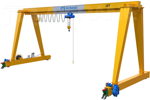
The System Model
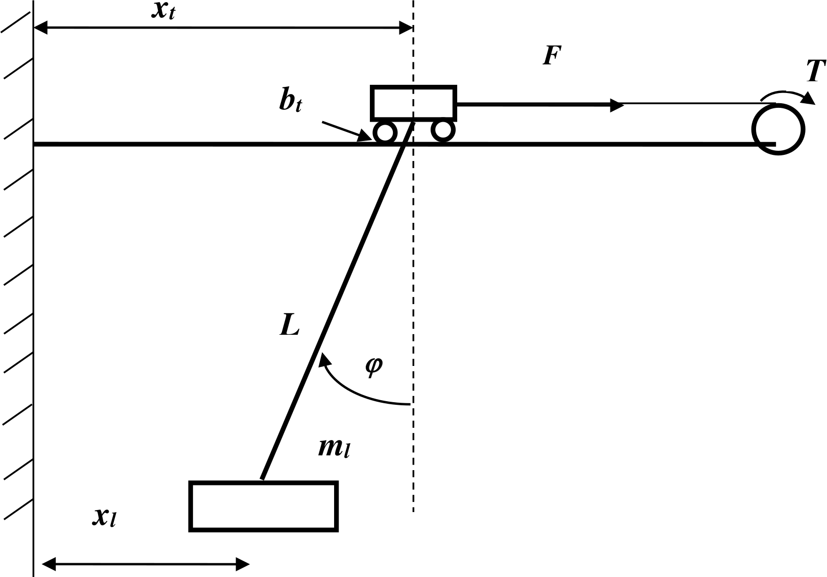
In our project we were only considering the motion to be along a single axis, although an additional one can be easily incorporated into the system. The crane system consists of a trolley, rope, and payload. These are shown modelled in the figure below, where:
\(m_t\) – mass of the trolley
\(m_l\) – mass of the load
\(x_t\) – horizontal displacement of the trolley
\(x_l\) – horizontal displacement of the load
\(v_t\) – horizontal velocity of the trolley (\(x_t’\))
\(v_l\) – horizontal velocity of the load (\(x_l’\))
\(\phi\) – angular displacement of the rope
\(L\) – length of the rope
\(b_t\) – coefficient of friction between the trolley and the rail
\(b_l\) – coefficient of friction on the load (caused by pivot joint friction and air friction)
\(F\) – force applied to the trolley
Fundamentals
This task had us list several potential input and output variable pairings for a feedback system from how the crane was described, for example \(F\) as an input and \(\phi\) as an output. We then had to explain the purpose of such a closed-loop system and how they would improve the crane’s efficiency. This came down to stating that we needed a closed-loop control system because we were aiming to control \(\phi\), but it cannot be controlled directly, only as the result of other system features.
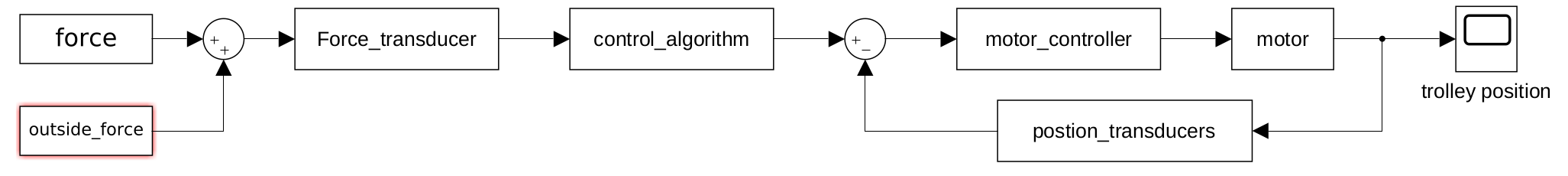
In addition to outlining our fundamental understanding of the control system we needed to develop, we had to prove it by making a generic block diagram of one input-output variable pair, showing a potential disturbing signal and other typical components of a flow diagram. I selected to do \(F-x_t\).
Modelling
The next stage of the project was to derive the mathematical models fo the system by hand and use them to find some transfer functions between key inputs and outputs. The mathematical models for the system were:
$$ x_l = x_t - L sin(\phi) $$$$ g\phi m_l = x''_l m_l + x'_l b_l $$
$$ F = x_t m_l + x_t b_t + gm_l tan(\phi) $$
To make things easier for us as we made the transform functions, we were allowed to linearize our models by assuming that \(\phi\) would in most cases be approximately zero, thus \(sin(\phi) = \phi\) and \(cos(\phi) = 1\). Our new model was:
$$ x_l = x_t - L\phi $$$$ g\phi m_l = x''_l m_l + x'_l b_l $$
$$ F = x_t m_l + x_t b_t + g\phi m_l $$
My generalized transfer function for \(\phi(s)/x_l(s)\):
$$ \frac{s^2m_l + sb_l}{s^2Lm_l + sLb_l + gm_l} $$My generalized transfer function for \(\phi(s)/v_t(s)\):
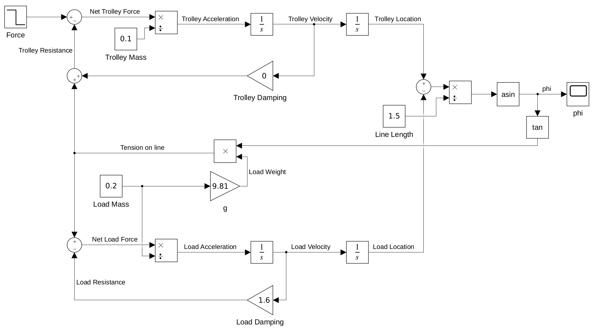
$$ \frac{sm_l + b_l}{s^2Lm_l + sLb_l + gm_l} $$I then entered the values I supposed to use for the various constants to get my final answer for each transfer function. After all these hand derivations, I then turned to the last component for this task, generating a Simulink model of the crane based on input force.
Transient Time Response
This was a short task that focused on having us simulating the transient response of \(\phi(s)/v_t(s)\) to a step and ramp input, with an open loop and negative unity feedback, for a total of four responses plotted.
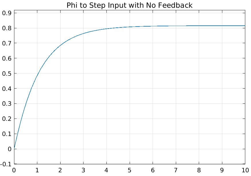
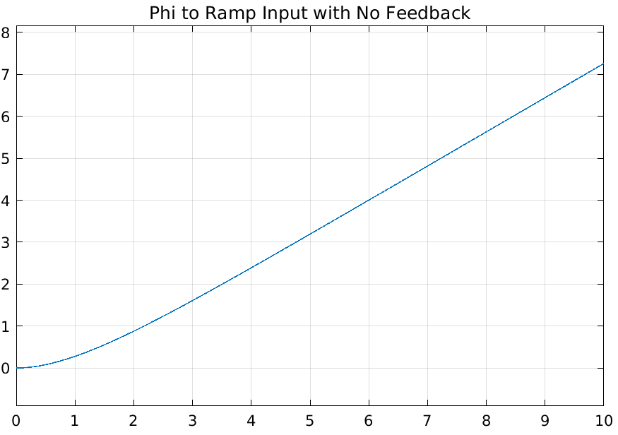
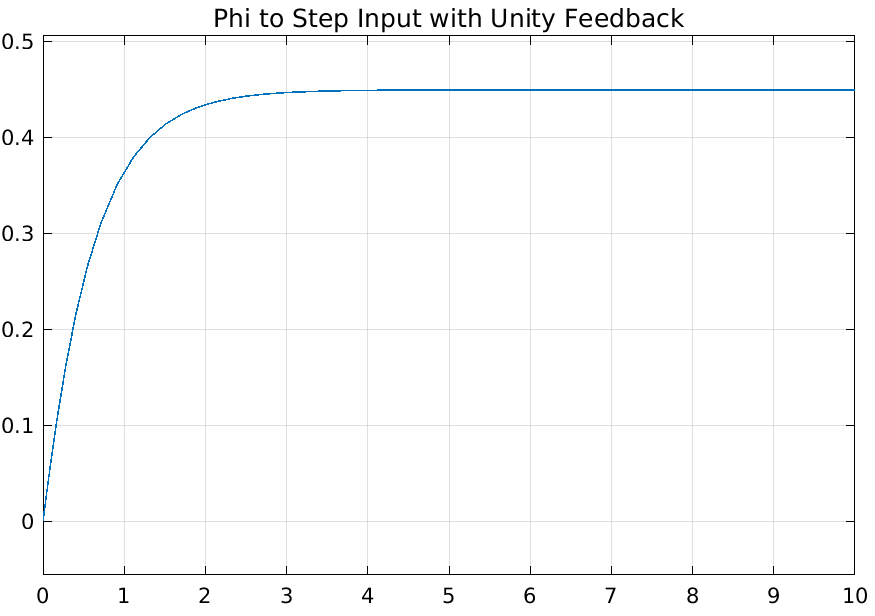
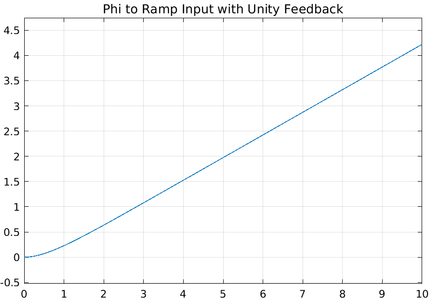
As we can see, implementing a unity feedback did effect the output. However I feel that this is not an appropriate feedback system since we are doing a difference of two different units to get an error signal, speed and angle.
The final part of this task required us to suggest a location for a controller in the negative unity feedback system. My suggestion was to put it between the error signal and the transfer function as this is the place I felt lent itself to be best tuned. Although I believe it would have been equally, if not actually better in retrospect to place it on the feedback line to the error calculation to convert the angle into a speed unit to generate a “proper” error signal from the difference of two speed values instead of an angle and speed. However this was outside the scope of our class (we were only learning about negative unity feedback).
Design
The final stage of this project was to top all our effort off with a properly designed controller for the system. First I needed to determine the stability of the system using the Routh-Hurwitz criterion, and then go forth to design the controller using a root-locus plot. My final proposal needed to maintain a percent over shoot (POS) less than 1%, and a settling time (\(T_s\)) less than 0.45 seconds.
Stability Check
To determine the stability of my system, I used the using the Routh-Hurwitz criterion. Using my parameters for the system (the masses, resistance, etc.) the following transfer function describes the system:
$$ T(s) = \frac{0.2s + 1.6}{0.3s^2 + 2.6s + 3.562} $$This transfer function generates the following Routh table. Going down the first column of the table there are no sign changes as all terms are positive. This means there are no poles in the right half of the imaginary plane, leaving both poles in the left half, thus the system is stable. I will not got into the theory on this, please check the link for a proper explanation if you are interested.
| s | ||
|---|---|---|
| \(s^2\) | 0.3 | 3.562 |
| \(s^1\) | 2.6 | 0 |
| \(s^0\) | 3.562 | 0 |
Actually Designing a Controller
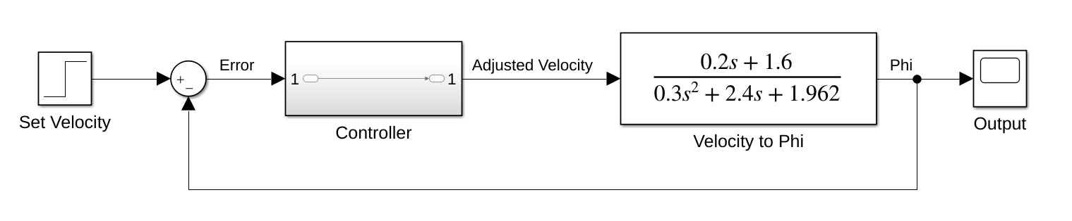
To use the tools in MATLAB and Simulink to help me tune my system I had to start by inputting my system’s transfer function into MATLAB and then call Sisotool to allow us to view and edit Root locus diagrams. This was done with the code below.
s = tf('s'); % Used to define function

% Define transfer function and output to terminal
g = (0.2*s+1.6)/(0.3*s*s+2.4*s+1.962)

sisotool(g) % Open sisotool for this system
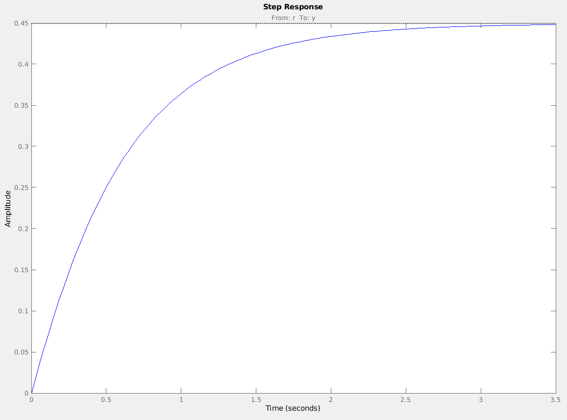
This would generate the familiar step response of the system…
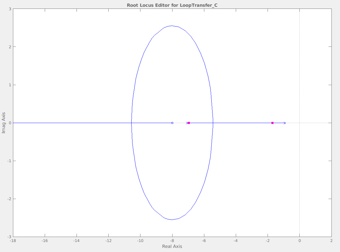
… as well as the Root-Locus diagram. The root locus helps us see where the current system’s roots are, and then lines/curves of where they could be as we vary the error gain, K. In the figure below the current roots are marked as pink dots on the blue lines of possibility.
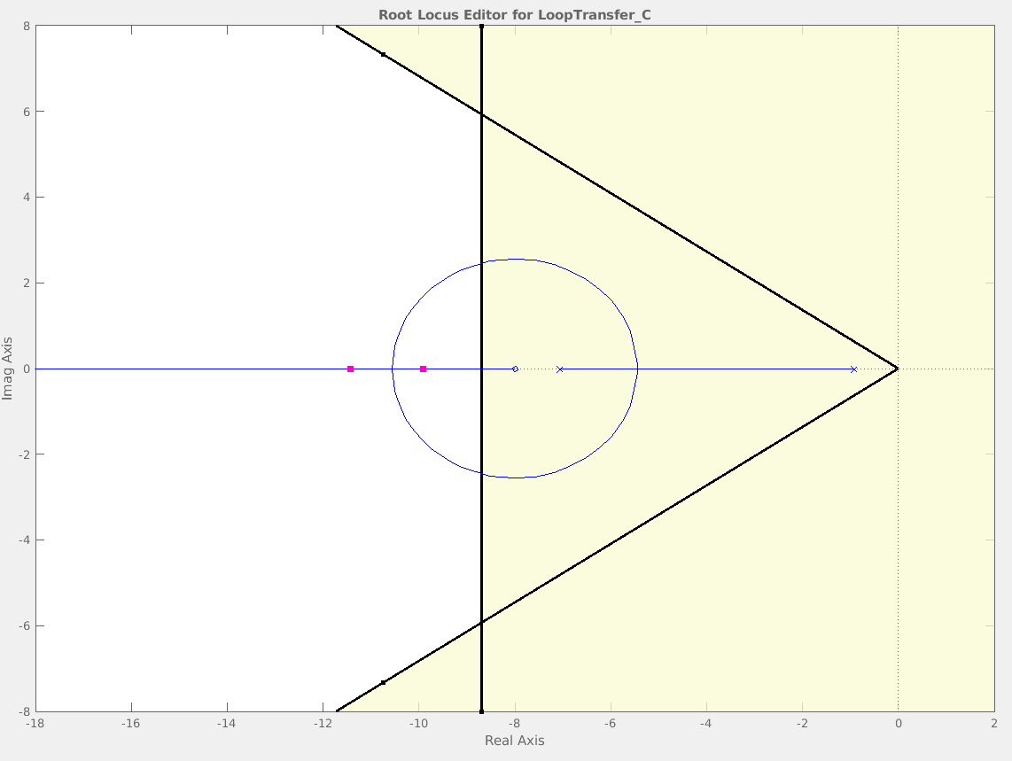
With sisotool started, I added the design requirements to the root locus graph. This added shaded regions that the dominant roots needed to be out of to satisfy.
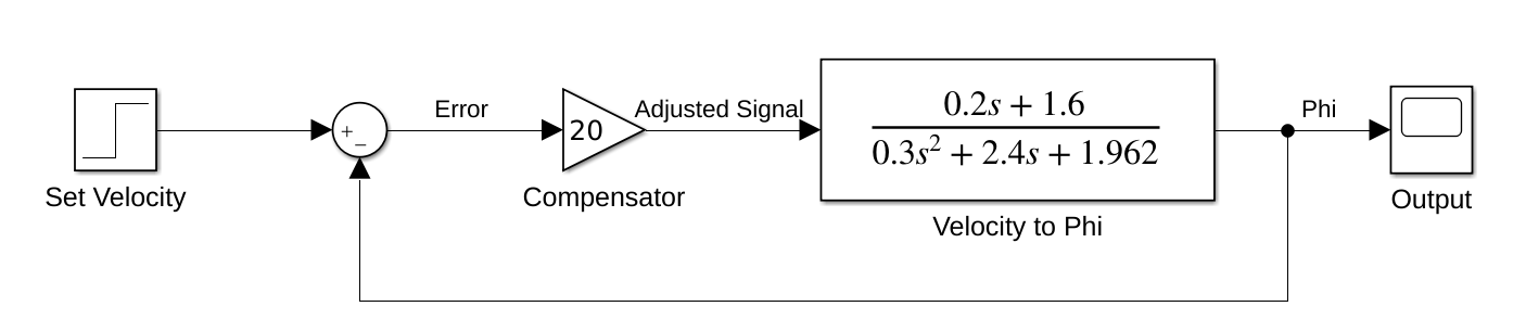
I arbitrarily selected 20 as the gain to see if it would meet these criteria. Lucky for me it did, and below we can see the unit step response for the system when K is 20. Although I had a working answer I did play around with K to see how the roots would more and the transient response change.
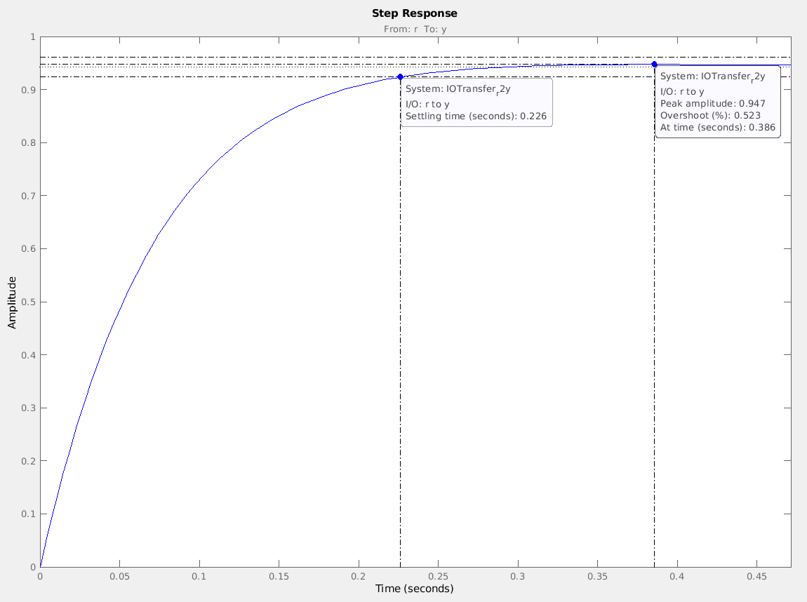
This led to my proposed system being the following:
Reports
This page is basically a retelling of my work presented in the two reports. Although I believe a better job of making my work easier to read with this web page, I know that I stripped much of the working that went into this as well as the nicely formatted math in the reports. You can find the reports at the following links:
Please note that these reports were written in response to a set of questions and not in a typical “report” format.