Overview

A major component of MIE444, Mechatronics Principles, was the project of designing and programming a robot in a team and having it autonomously navigate a maze to find and retrieve a block. My primary technical contributions were in the circuit design and programming for my team’s project.

Since the course was being delivered fully online we merely proposed our teams' designs and one was selected and built by the instructors which we than submitted algorithms to operate that we developed using simulators and some limited testing on the actual robot.

In addition to delivering a design proposal and control algorithm (written in MATLAB) we were also required to submit a final report explaining our algorithm.

Requirements

• Design a rover to do the following:
  1. Move within a maze without striking any obstacles
  2. Localize itself and plot a path inside a known maze
  3. Find and pick up a block
  4. Return with the block to a predefined end zone
• Design the control algorithm in MATLAB using the allowed instructions to interact with the robot
• Submit a design proposal and final report document and presentation
  • Design had a budget limit of $300

Objectives

• Minimize collisions
• Use a flexible path finding algorithm instead of hard-coding paths
• Move as quickly as possible

Takeaways

• I learned how to implement and use path finding
• Exercised my ability to design mechanical mechanisms
• Practices technical report writing
• Developed an ability to identify specific test cases to validate features
• There needs to be a balance between offloading too little or too much computation.
  • For example obstacle avoidance could have been implemented on rover to save time

Detailed Report

For one of my courses in my final year of undergrad I took MIE444 - Mechatronics Principles. This class had a project that was to build and program an autonomous rover to navigate a maze and retrieve a block in groups of up to four (I worked in a group of three). The project was broken down into five assignments: two reports and three contests for functionality. The order of which were:

1. Rover design proposal (report).
2. Obstacle avoidance. We had to move the robot about 7m within the maze, losing points per collision or for not covering all 7m in the time frame.
3. Localization and path finding. Rover would be placed in the maze, need to localize and navigate to a predefined location.
4. Block retrieval. Robot would be put in the maze, need to localize, navigate to the block zone, pick up the block, and take it to the designated end zone.
5. Final report.

The spacing varied a bit between assignments, but was generally about two weeks. For the three contests (2-4) our only deliverable was the code required to operate the rover.

Since this course was delievered entirely online, we did not build or program our own rovers. Instead the course team had us vote on all our submissions and they made a hybrid of the design which received the most votes (not ours). We then developed our code to operate these using simple commands to exchange data with the rover, such as “move forwards this much” or “sensor 4 reading”.

Design Proposal

Our proposed rover was based on a holonomic drive allowing it to move in any direction relative to its orientation. This was to be provided by three independently driven omni-wheels at 120° around the base. Atop the base sat the battery and our gripper mechanism. The gripper was operated by a single servo motor to both pick up and then release the block. The top layer housed all the control electronics and most sensors (excluding one ultrasonic sensor used to detect the block).

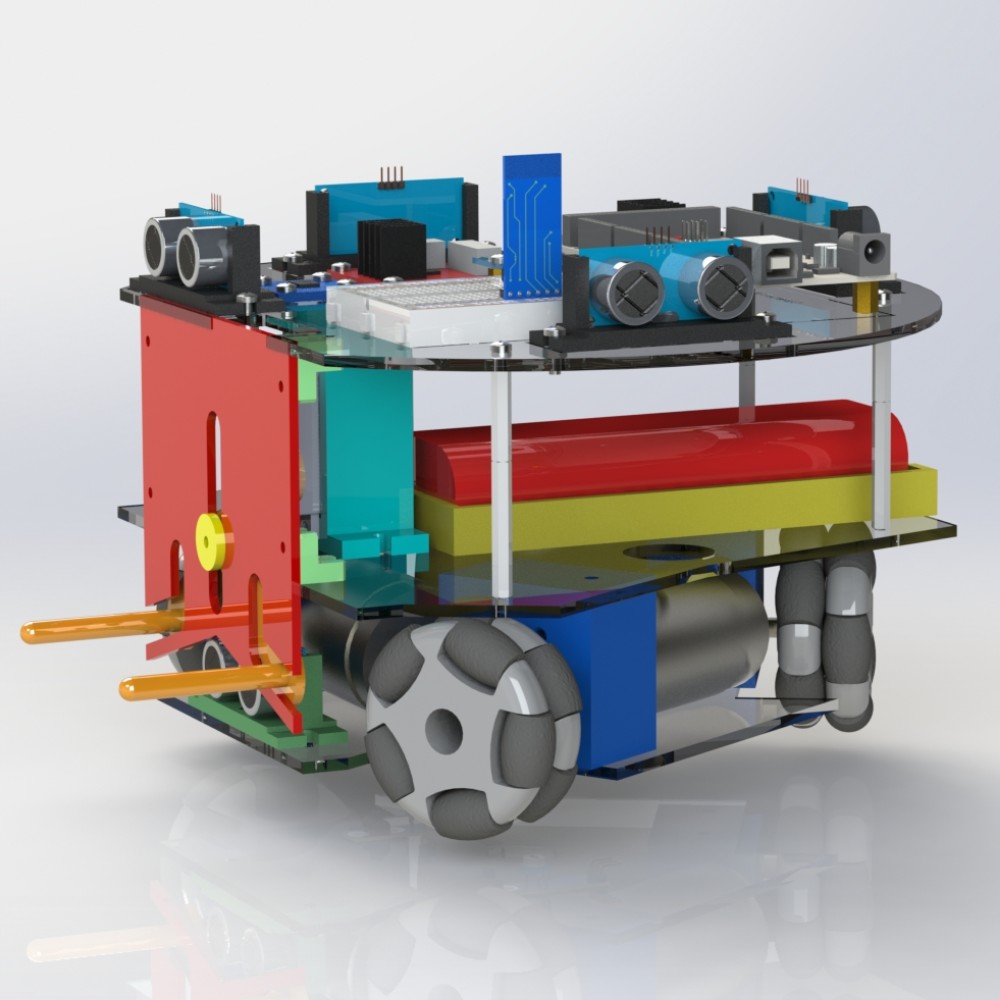
The reason for this layered design was to make use of the light manufacturing capabilities available to us as students in making an easier to assemble and maintain rover. The primary manufacturing equipment being 3D printers and laser cutters.

For this design proposal I had two main contributions, the circuit design and the gripper. I wrote their related sections in the design proposal report as well, which you can find here.

Gripper Design

Our gripper design had several constraints on it, largely due to our choice of drive train taking up a considerable portion of the available footprint. We also wanted to minimize the degrees of motion to ideally just one to simplify the system and its control. This meant that we needed to find a way to both lift and hold the block in a nearly vertical space.

I came up with the design we proposed that should have achieved this. It was a linkage system driven by a single servo. As the servo would rotate its arm, it would move on joint vertically in a guide on the front plate. This vertical motion would be further transmitted to the two “arm” links that will then squeeze the block and pull it up as they follow their guides in the front plate. These “arms” were meant to be wrapped in rubber to improve grip compared to bare plastic.

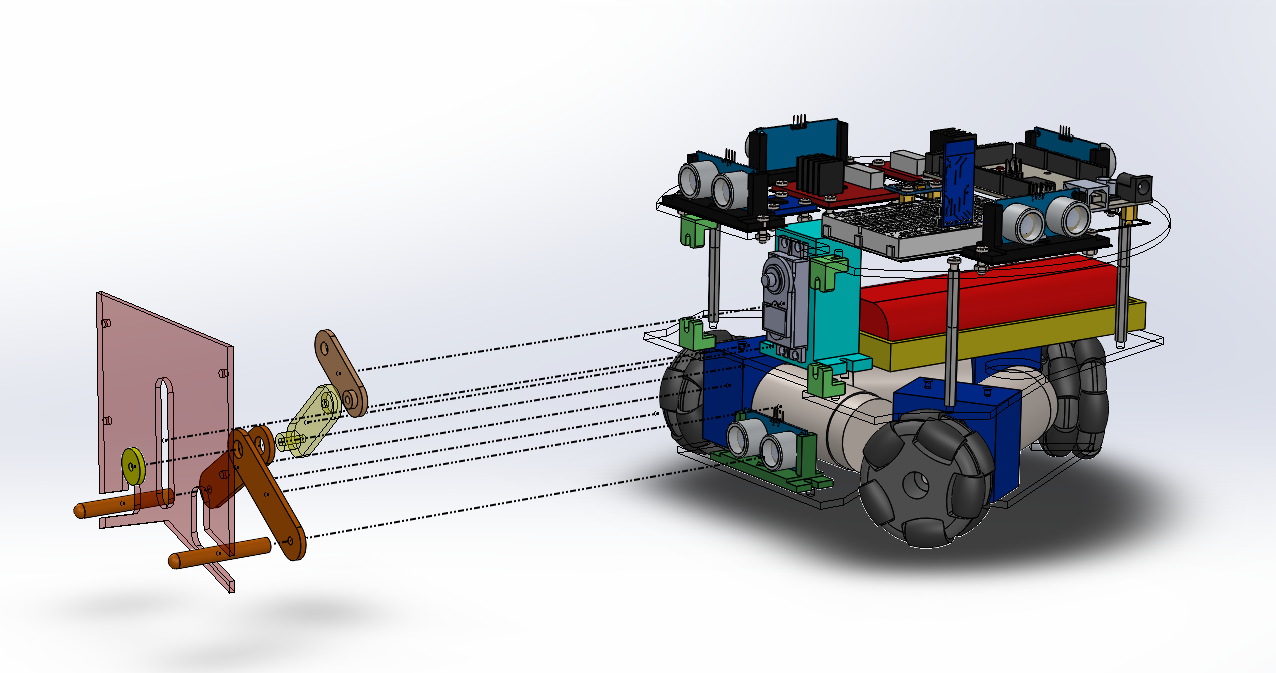
To release the block, the system would simply be driven in reverse.

Circuit Design

I designed the entire proposed circuit to drive our rover. At the heart of is was an Arduino Mega, used for its numerous inputs and outputs available to us. This would allow us to write code that would operate the entire robot from a single microcontroller.

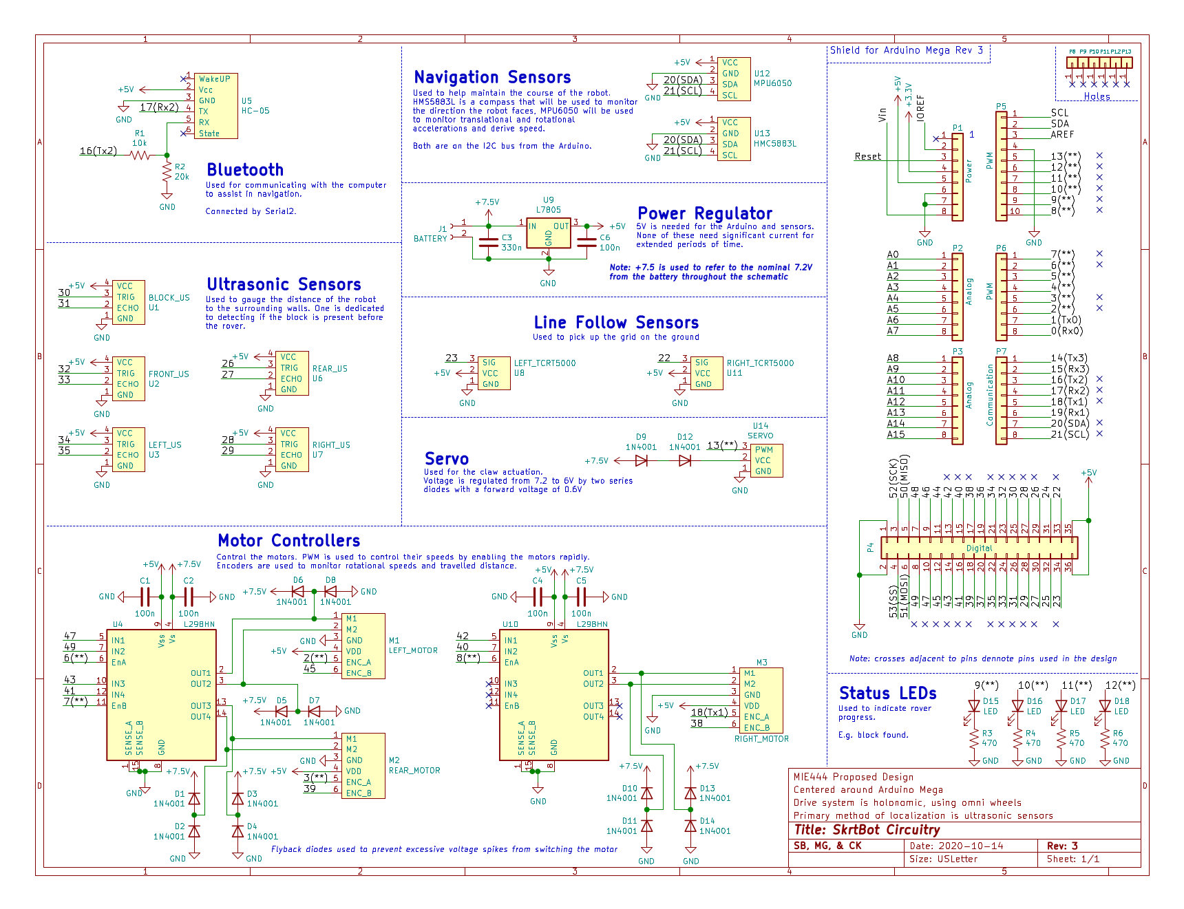
Inputs

The rover had many inputs to help guide it.

• Bluetooth communication was needed to link with the computer where the high level computations were handled.
• Ultrasonic sensors used to determine the distance to adjacent walls and the presence of the block
• Line follow sensors used to pickup the grid under the rover as it travels to aid in localization
• MPU6050 IMU used to help ensure the stability and fluidity of motion, potentially displacements
• HMC5883L compass used to help maintain the rover’s heading
• Encoders on each wheel to monitor rotational speed

Outputs

The rover had a few outputs, primarily related to motion.

• The three base motors to move the rover (driven in pairs by L298HNs)
• The gripper servo
• Four status LEDs

Layout?

Since I knew that if our circuit was going to be chosen, it would most likely be recreated on a breadboard I didn’t bother to lay out a circuit board for it. Perhaps I would have if our design was chosen, at least one to get milled on campus but alas we will never know.

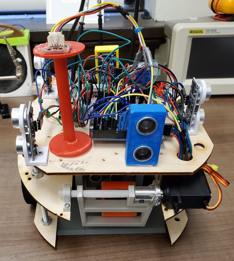
The Selected Rover

The rover the class selected was a fair bit different to our proposed design. I will summarize it so it can help explain the choices we made in our algorithms.

• Differential steering base (like vehicles with tracks)
  • Stepper motors used for more accurate and repeatable motions
• Five ultra sonic sensors on the top for wall detection (two shared a side to help determine the rover’s alignment to it)
• Compass module
• Box grabber was essentially a scoop and ramp, with an ultrasonic sensor to try and spot the block

Control Algorithm Development Process

Once the rover was selected and built for the class, we started preparing code to operate it. Our code had to be written entirely in MATLAB script since that was the framework the teaching team was using to operate the rover. (Had we been building our own rovers it would be left entirely up to us what we use.) Other than the script the prepared for us to use to exchange data with the rover and the rover command structure itself, the rest of our code was up to us.

Note: I initially wanted a more modularized approach, with each function or group of functions in its own file, however for the sake of simplicity when submitting we used one large script

A typical exchange with the rover would appear like this, with us specifying the commandString (s_cmd and s_rply were set when the Bluetooth communication was started):

sendCommand(commandString, s_cmd, s_rply); % Just sending a command string
                                           % No interest in response, used mainly for motion

readings = sendCommand(commandString, s_cmd, s_rply); % Record the response to 'readings', used for sensors

The command string format was a two character command type, followed by a quantity, seperated by a dash ("-"). For example the command to read all ultrasonic sensors five times and return the average reading for each was ua-5 or to rotate 45° left was r1--45 (negative 45 since left was marked as negative, right was positive).

All the embedded, rover-side programming was handled by the teaching team, so we only worked on these algorithms to navigate, and not low level stuff like the process of collecting ultrasonic readings.

Simulations

Since we did not have access to the rover or the labs at all (compared to previous years where students built and kept the rovers themselves and the lab with the maze was accessible 24/7) we primarily developed and tested our algorithms in simulations.

There were two simulations available to us, one written by the team in MATLAB that they used in previous years to help people develop their navigation code without the hassle of hardware issues and a more complicated, but physics-accurate 3D one. Our team stuck to the simpler MATLAB one since we felt it would provide us a reasonable representation of how our algorithm would behave without taking too difficult or long to run.

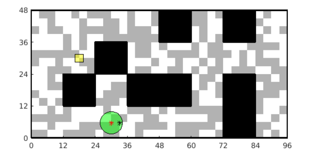
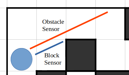
The MATLAB simulation was a top down view of the maze with the block and the rover present. The rover was represented by a light green circle and would be commanded around in the same way the actual rover would be. There was also collision detection and simulated sensors. The ultrasonic distance measurements are shown with red lines extending from the rover.

Testing in Reality

Although our primary method of testing our code was the simulations, we did have some days leading up to each milestone where the teaching team would set up in the lab and run code teams would submit. And we would watch over stream the rover’s motion and the terminal output from MATLAB (useful for debugging what went wrong when watching replays).

Generally most teams would have two scheduled runs a day and then there was free time at the end for teams, especially those that had issues earlier, could go again.

Obstacle Avoidance Milestone

The first milestone simply required us to get the robot to move though 20 blocks (20') within our 8 minute limit, there were no designated points for it to visit as it wandered.

For this task the general flow of the program was to have the rover aligh itself with either primary axis of the maze, and simply move forward until it could no more, then turn left, right, or backwards depending on which was available, repeating until it was stopped.

Alignment

Initially I wanted to use the compass to be the primary sensor to monitor alignment since the maze was always aligned East-West along the longer side, thus I could always find the different between the rover’s heading and the desired one to use as a corrective angle. We could use difference in ultrasonic readings on the right to corroborate this angle. In the simulation this worked fine, perfectly really, as shown in the figure below.

In reality the story was quite a bit different. I had written into our first set of code to be run on the rover to have the rover spin in place a few times, recording the compass readings every 45° so I could verify which direction was which heading. Our instructor had warned us of the issues with the compass and they were clear here. The measurements were not at all what I expected, neither repeatable nor linear with motion (some 45° turns changed the heading returned 120°, others only 15°).

This dissuaded us from using the compass and we instead solely relied on the ultrasonic sensors to maintain alignment for this milestone.

We did later return to using the compass for other milestones when a classmate told us that they had fixed the issue. I believe it was something to do with the calibration of the sensor that was at fault.

Obstacle Avoidance

Alignment was the first piece of the puzzle for obstacle avoidance, since if we were aligned with the maze and there was nothing in front of us, we could confidently move forward and not worry about hitting a wall (as long as the front facing ultrasonic sensor didn’t see anything). Compare this to if the robot was at 45° to an axis and the rover looked forward, the ultrasonic sensor might not see a wall in front of it but the rover may drive forward and collide with a corner.

To develop on the alignment my teammate developed a “lane” system for the rover. The rover would use the ultrasonic sensors on its sides to determine how centred it was in its “lane” if it was too close to either wall a corrective motion was added to the next forward step. For example if the rover needed to move a centimetre away from the right wall, the algorithm would do the trigonometry to tell the rover what angle left to steer before moving forwards.

The combination of alignment and “lane” control performed favourably in the simulations, with only very rare collisions.

When tested we were able to traverse the 20 squares in under six minutes, with only two collisions!

Localization and Path Finding

The bulk of my effort in this project went into preparing the algorithms for this milestone. My teammates worked to prepare convenient moveForward and setHeading function I could call in my navigation script that would bundle all the obstacle avoidance code into function that would move the rover safely forward one whole square or set the robot to face a given heading respectively. With those abstractions I could focus on the higher-level control.

The layout of the maze (including pick up zone and drop off point) are known in advance and do not change! The only unknowns for the rover are its starting position and orientation, and the exact location of the block in the pick up zone.

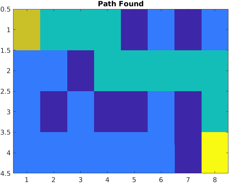
Path Finding

I started with path finding because it was probably going to be easier and also because I had been working on some [unfinished] MATLAB code to do it in 3D for my capstone. It was also easier to test since I didn’t need to test with a simulation, I could just enter start and end points.

Although hard-coding four sets of paths (one to the pick up zone, three different drop off) was feasible in this application, I felt that it would be more interesting and educational for me to use something procedural that I could apply to my capstone as well. After some research we decided on using the A* Algorithm for path finding. For the cost heuristic I used the “Manhattan” distance between squares (moving along axes, not a straight line).

Implementing this was pretty basic and it worked like a charm after a couple of tests.

Localization

For navigation we decided to use each square as its own node in our map since we we confident we could move the rover reliably from one square to the next and we wouldn’t need to localize mid-motion. Some of our classmates did however opt for more granular localization - subdividing each square into sixteenths (the size of the markers on the ground) or smaller.

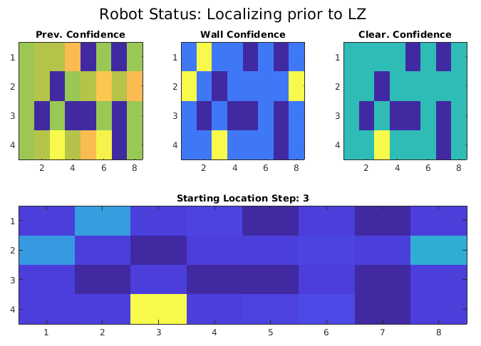
Localization was not meant to be absolute, rather a probability of where the rover was in the maze. Given the sensors available on the rover, there were three factors that could be used to contribute to an estimate of the rover’s location:

1. The immediate (blocking) walls
2. The distance to walls (clearance) on each side
3. An estimate based on the motion performed applied to the previous confidences

Each one of these factors is calculated for each node in the maze, and then they are combined using a weights for each factor to produce a final estimate.

History Based Localization

The simplest of the factors to calculate.

0. The confidence map at the end of each turn is saved
1. All the values are shifted to match the motion of the rover since then
   • The heading of the rover was confirmed using the compass which was working properly at this point.
   • E.g. moving one square towards the left would shift all the previous probabilities to the left.
2. Apply a mask to nullify any impossible positions (inside an obstacle, out of bounds)
3. Set the the end row or column that was “pulled in” from outside the maze would be set to zero.

Wall Based Localization

This is the most basic localization available when using wall clearance data. If there was a wall detected within a short distance of the rover it would be marked as a one, otherwise a zero. These values were strung into four digit number going around the rover: front, left, rear, right. So if there was a wall to the front and right of the rover, “1001”. Each square in the maze would have some variation. The map below shows these values for each tile starting from the top going counterclockwise (as though the rover were facing the top).

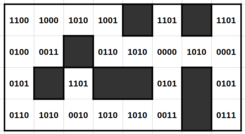
By having the values stored in this sequence it allows the algorithm to shift the letters left or right to match a potential square even if the rover’s heading doesn’t return the exact same string. For example “0110” and “1100” could be returned the rover at the same square, the only difference being the heading of the rover when it recorded it.

Distance Based Localization

This was essentially an upgrade of the wall-based localization estimate. It worked in the same way to guess where the rover was, except instead of using information on which sides walls are blocking the rover, it used the number of squares to a wall on a given side. A zero would be used for any blocked sides, and then counting up. The algorithm would use the ultrasonic readings, divide them by a square’s length and round to determine the number of squares in any given direction.

As you can see in the clearance constants map below, this leads to far fewer repeating IDs and thus quicker localization.

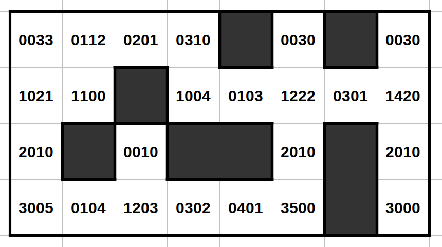
One problem that emerged with this method (hence why it wasn’t the only method used) is that poor sensor data especially results around the threshold of a square being counted or not would cause some bad estimates, and given the uniqueness of most tiles this would often significantly mislead the rover and take a long period of time to re-localize.

Combining Factors

Tee factors were each scaled by some factor (a power) and then multiplied together to generate a combined estimate, which was then normalized. Balancing these weights took me longer than I expected.

Since this was a probability distribution, we needed to define a threshold for when we would declare the rover localized. This ultimately was a two part threshold: an absolute confidence threshold (e.g. 0.30) to be in a given square, and then a relative one between the top two confidences (e.g. top estimate’s confidence must exceed the second best estimate by 50%). Once these were both met the robot was declared localized and then the data would be used to start path finding and follow the steps to the destination.

Ultimately because of the aforementioned sensor issues and poor weighting, we met expectations, but did not excel in our localization trials. These issues were addressed for the final milestone with more realistic simulations and real world testing.

Grabbing the Block

Grabbing the block wasn’t too difficult in theory, but that’s how theory always is, isn’t it? The rover was meant to enter the pick up zone and face away from the middle. It would then begin to incrementally scan across the zone for a difference between the two front facing ultrasonic sensors. If the block level one detected an obstacle notably closer than the top one, chances are that it would be the block.

Instead of immediately stopping and going to grab the block, the rover would continue to scan until the block was no longer detected. It would then go in the middle between the start and end of where the block was detected, effectively centreing it and then approach partially.

It would repeat this process at least once more because doing partial approaches prevents the rover straying far off course.

Note: the MATLAB simulator did not have physics for the cube, hence why it does not react to the rover colliding with it.

In reality we had come issues with the reliability of sensor data due to the partial misalignment of the front ultrasonic sensor as well as the general nature of ultrasonic obstacle detection. A notable corner case is when scanning and passing one of the corners of the loading zone causing occasional false positives.

Fortunately in one of our trials we didn’t have any issues, and got a perfect score

Final Report

The final report was meant to be a summary of the work we did for the three milestones, explaining the algorithms we used and justifying our choices. I’ve reused much of it to make this page, albeit focusing on what I worked on. You can read it here as a PDF.

We also had to submit the code we used in our final milestone test. All 1300 lines of MATLAB viewable here.