Rescue Rover
Table of Contents
Overview
For my class “MIE444, Mechatronics Systems” we had to develop a control algorithm that would eventually be deployed on a robot to aid the victims of a simulated disaster. Unlike the project for MIE443, the mazebot, the focus was solely on the algorithms (no hardware design) as we would be deploying on a standard commercial robot kit called the TurtleBot2. These algorithms had to work within the Robotics Operating System (ROS) framework.
The project had three milestone for which my team of three had to submit both code to control the robot, as well as a report explaining and justifying our choices. We each had to submit a small report individually for these, answering a couple of questions. The milestones were:
- Obstacle avoidance and exploration/mapping
- Image detection and path planning
- Emotion detection and emotional control schemes
These contests/milestones would be developed and assessed in a virtual environment built into ROS due to the fully online structure of the course due to the pandemic. Previous years would actually use a physical TurtleBot2.
Overall our team was successful at achieving all milestones. My primary contributions were coding the image and emotion detection and processing, the movement code and writing the related sections of the reports.
Requirements
- Milestone 1:
- 15 minutes to explore and map 6 by 6 m area with static obstacles
- Speed limited to 0.25 m/s in open space, 0.1 m/s when near obstacles
- Must use sensors for navigation (no preplanned motions)
- Milestone 2:
- Visit the location of each tag and identify it
- 8 minute limit
- Milestone 3:
- Use machine leaning to identify the emotional state of disaster victims based on facial expression
- React differently to seven different emotions
- Explore and map unknown area, searching for victims with unknown locations
Objectives
- Milestone 1:
- Minimize collisions
- Explore the entire available space before hitting the time limit
- Produce an accurate map
- Milestone 2:
- Optimize path planning to reduce movement time
- Maximize the accuracy of identifying tags
- Milestone 3:
- Find all the victims in the time limit
Takeaways
- Working with establish libraries and frameworks is quite fun
- ROS is a very interesting framework to work in and I would enjoy returning to it
- Image processing isn’t as hard as I thought it would be using OpenCV
- Emotional control schemes for robots are an interesting and understanible way to implement complex behaviours
- The importance of having robots signalling intent when working around/with people
- Image pre-processing is vital to good recognition
Detailed Report
MIE443, Mechatronics Systems was a project based class I took in my final semester of undergraduate studies. My grade came entirely from the project with each of the three contests/milestones weighed equally. The project was to develop the control algorithm that operated within Robotics Operating System (ROS) for a standard commercially available robot kit called the TurtleBot2.
Each contest built on the previous so it was necessary that our algorithms were written properly from the start to avoid issues snowballing at the end. The milestones were:
- Obstacle avoidance and exploration/mapping
- Image detection and path planning
- Emotion detection and emotional control schemes
In addition to the performance of our code, we needed to submit a report with each milestone which was worth half the marks. These reports would need to detail and justify the choices we made and the work we produced.
Robot Overview
The robot used for this project was a TurtleBot2. It was composed of a Kobuki base which everything sits on and a hardware frame atop it. The default robot like the ones we were using come with a first generation Microsoft Kinect sensor and a laptop to operate the system.
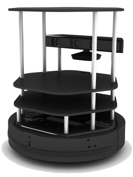
It had significant support in ROS provided by the vendor so getting to work with it was quite simple.
Inputs
The robot had a few different input channels available for use:
- Kinetic Sensor
- RGB Camera for vision
- Depth (distance) image provided by infrared scanner
- This was also used to generate a “laser” field with the shortest distance to anything at a given heading for the robot
- Kobuki base
- Odometry with 52 ticks/enc rev, 2578.33 ticks/wheel rev, 11.7 ticks/mm travel
- Gyroscope for monitoring rotational speed up to 110 deg/s
- Bumpers on the front side’s left, centre, and right
- Cliff sensors on the front side’s left, centre, and right
- Left and right wheel drop sensors
- 3 touch buttons
Note that not all of these were used in our project, given the flat and virtual operating environment we had no use for any of the sensors listed past the bumpers.
Outputs
The robot had fewer methods of acting on the environment than reading the environment. Other than moving the robot itself, the laptop could be used play multimedia on command using its built-in screen and speakers.
Rereading the Kobuki base documentation now has informed me that there were two RGB lights available to use on it, as well as a basic buzzer but neither of these were mentioned during instruction - likely due to the virtual nature of the project.
Coding Overview
Each one of these acted as an introduction to a new tool and/or code-base which made for a gradual and connected learning process as we started using each tool with the previous ones immediately instead of just writing programs separate of one another. The order we were introduced to tools was:
- ROS, to control the robot
- OpenCV, to do computer vision
- Python and TensorFlow, for machine learning
The main IDE we used for ROS and OpenCV was VS Code. It had built in version control features which were necessary for this collaborative project. The vast majority of code we prepared was written in C++. When working with TensorFlow and Python, Google Colab was used instead as it offered (limited) free run time on their servers with GPU accelerations for training. By training on their servers compared instead of our computers, we were able to train almost 10 times as fast!
Testing and Simulations
As mentioned before, all my courses in my final year of undergraduate studies were delivered online due to pandemic restrictions. This meant no access to campus for students and so all our developmental testing had to be completed in simulations, luckily ROS has a built in utility for this and the TurtleBot team prepared what was needed to make use of it. Unlike with the the mazebot, the algorithms we prepared would be assessed on its performance in the same simulation used for development. Not running on a real robot. I felt this was fairer to the students since many of the issues we faced in MIE444 were related to sensor issues that were difficult to diagnose and iterate on remotely.
This simulation software was called Gazebo and was a full 3D simulation, with proper physics for collisions and such. It was able to properly simulate all the appropriate sensor data streams too, including even the camera feed! In the figure below I took a screenshot of the simulation in progress, from left to right: simulated camera feed (over a window of VS Code), visualization of the robot’s generated map with it’s estimated position and path finding overlaid, the Gazebo window for the whole simulation showing the “true” world.
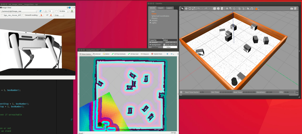
It felt really cool when simulating the later labs and there would be a half dozen or more windows strewn about for the simulation alone. Good thing I invested in a decent amount of RAM for my PC.
Milestone 1 - Navigation and Mapping
The first milestone was pretty basic, we had to design a control algorithm that would basically have the robot wander on its own and map the surroundings as it went. The goal being to have it explore and accurately map as much of the environment as possible within the time limit.
ROS
The Robotics Operating System is a massive open-source project designed to accelerate the development of robotics control systems by providing standardized software interfaces for all sorts of hardware and software to work within its framework. Unlike my experience with embedded projects where everything had to be operated by a single process or thread, ROS makes use of multi-threading available on modern computers and thus most components each run as their own thread. Even the different parts of the robot run as separate process that others can subscribe or publish to to begin exchanging information.
This meant my team and I had to familiarize ourselves with the structure of ROS and how it works, for example writing code that would “publish” instructions to a “topic” instead of calling a function to move the robot. Likewise setting up other code blocks to “subscribe” to topics like the bumper to handle us colliding. Most blocks of code (modules) did some of both.
Although ROS has support for C++ and Python, and we had the option to use either, our team choose to use C++ since we were more familiar with it.
Movement
Once we were familiarized with the basics of ROS we went on to prepare our exploration/movement code. We would be operating the robot at a low level, issuing commands directly to the base for motion and reading in sensor information directly.
We adopted a modular approach coding functions that would interact with the robot, such as telling it to move, and others to collect information from the robot. We then made larger functions that called upon these to do more complicated things, such as moving a specific distance using feedback from the sensors, or turning to face a particular direction.
The resulting functions that we created were setHeading and travel. setHeading would set the robot’s heading to whatever was passed to it, like 0 for North. travel on the other hand was used to move the robot to complete a desired displacement both linear and rotation, at desired rates. Using these two functions made our main code simpler to read and easier to maintain since all the feedback loops were in one place.
Mapping
Mapping didn’t actually need anything from us. Once started, ROS’s built in “gmapping” service would simply collect all the relevant data it needed from the robot and begin to create a map and localize the rover within it.
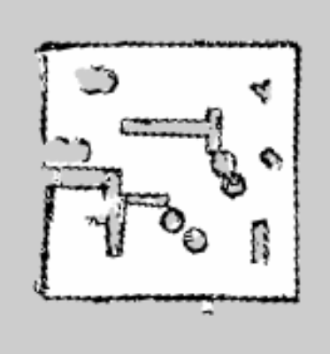
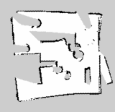
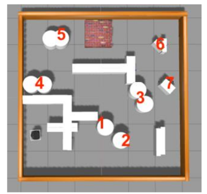
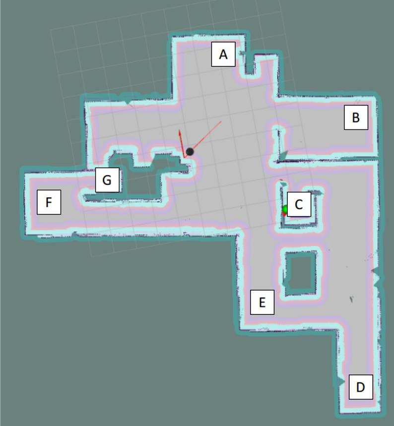
We did however need to accommodate it with our motion planning. For example moving too quickly would not produce enough data for an accurate map, as would rotating quickly or frequently. Below is a comparison of the maps produced by manual operation to ensure a nice map, compared to the robot performing a purely random walk. In these maps white areas are open space, black lines are obstacles, and grey areas are unexplored.
Exploration
Initially, we were aiming to implement a frontier-based approach to exploration, as this would be sure to get the robot to explore into new areas faster. However, due to time constraints and unfamiliarity with gmapping and the ROS localization suite, we instead opted to use a weighted random walk method for exploration, utilizing a reward function fed by the turtlebot’s depth camera to help guide the robot towards open spaces in front of it.
This method was easier to implement, which was important given the limited time we had for each competition. Compared to a true random walk, the weighted walk generally guides the robot to travel further and faster, exposing it to more of its environment in the same amount of time.
One issue we identified with this approach was that it had a possibility to get the robot stuck going down a long corridor in the area or along diagonals of open space. To try and prevent this from happening, I implemented an occasional “scan” of the surroundings by having the robot complete a full rotation and select a heading from that instead of generally forward one.
Overall Structure
Holding all this together was a finite state control system with three states:
- Bumper - Used whenever any bumper is struck
- Explore - Do weighted random walk (default state)
- Scan - Perform a rotational scan and decide a new heading
These would have their own sub-states within them, for example when scanning, there would be a state for the actual scanning rotation followed by another sub-state to move to the selected state before returning to the normal explore state.
A full version of our code for this milestone is available at our contest 1 GitHub repository.
Contest 1 Results
We did alright in this trial, although our robot struggled in navigating the tight quarters and likely ended up looping in the same area as we warned was possible. You can read our written report here. In our defence the area used for marking was significantly more dense in obstacles than our practice area, these were also generally much smaller and thus harder to distinguish one from another.
Milestone 2 - Image Recognition and Path Planning
The second milestone was quite different to the first, focusing on the deployment of image processing and path planning. The goal of this contest was to have the robot go to and identify what image was displayed on ten boxes in the world. The locations of these boxes and the map were known in advance and no other objects would be present in the world. After visiting every box and trying to identify the marker present, it would return to its starting point and output a file with its findings of which image was on which box in text.
Movement
For this contest we were allowed to use the built in move_base function in ROS which handled all the low level work of commanding the base, reading map and localization data, and plotting a path to follow. It essentially made our first milestone’s code obsolete.
All we simply had to do was call it once with a destination in the world and then it would plot the course and react to any obstacles it would encounter in real time and use the map the rover had generated. It ran in a separate process than our main code so our code could continue running as the robot moved.
Path Planning
Given the constrained time to complete our sweep of the world it was in our interest to optimize our robot’s movements through all its stops to minimize travel time. This is the classic “Travelling Salesman” problem, and there have been many ways developed to solve this problem.
The simplest conceptually is “brute force”, where one goes and calculates the total distance travelled for every possible route (also called a “Hamilton circuit”) and then selecting the shortest one. This is guaranteed to provide the optimal route every time, however it is very computationally expensive with its computation cost being the factorial (x!) of the number of stops that must be visited. With five stops, 120 routes need to be calculated - with 10, 3628800.
The other method we considered was the “nearest neighbour”. As the name implies, this algorithm simply builds a route by selecting the nearest unvisited point to the start, and then repeating from that point until all destinations are visited. This is a bit harder to implement and is not guaranteed to find the optimal route, however it is significantly cheaper to compute as more stops are added since the number of computations grows at about x^2 with the number of stops. With five stops, 15 distance calculations are needed - with 10, only 55.
We decided to try and go with the brute force method first and switch to the nearest neighbour if it was far too slow. Our initial code to brute force took about a half minute to provide a route, a respectable time since there is a decent chance it would make up for it with the savings in movement we would get. To reduce this computation time further we made the choice to an “Adjacency Matrix” this was an 11 by 11 matrix with the distance between any two destinations stored in it (11 destinations are the 10 boxes and then the start/finish point). By calculating this in advance, we could replace the calculation for distance between two points in the loop (\(\sqrt{(x_1-x_2)^2 + (y_1-y_2)^2}\)) with a much faster lookup in the matrix. This dropped the time down to get the optimum path to only about 5 seconds! This was acceptable for us and we left it at that.
Distance Consideration
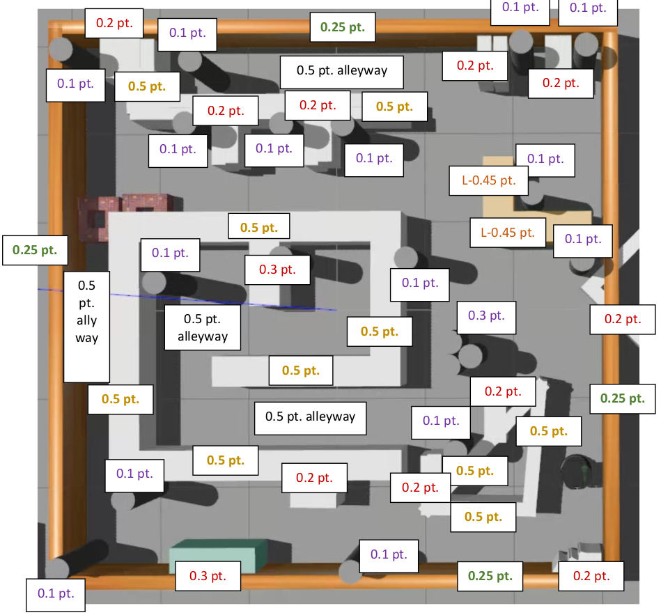
Looking back as I write this, I realize that using the direct distance between points as our “cost” value in these calculations might not have been the best way to do it. The reason being that the rover would be far more likely to encounter obstacles it would need to avoid and thus incur even more “cost” than expected.
I could have investigated how to pull the planned path length between two points as move_base would plot since the map was known to the robot in advance to get a more accurate cost. Another option if this was too difficult to do, is to simply apply a power to the distances between points before putting them into the adjacency matrix. This way, several medium length (and thus medium risk) segments would be favoured over a mix of shorter ones with a few long extremes.
Image Recognition
This was the bulk of the work for this milestone and I worked mostly on this for our team. We used the OpenCV framework which has been well worked into ROS, and thus easy to deploy for our project. The robot’s camera provided an RGB video feed at a resolution of 640 pixels wide by 480 pixels tall, at roughly 30 frames per second.
Our vision system needed to be satisfy the following for success:
- Differentiate between 15 unique possible images…
- Could be rotated
- Could be tilted towards or away from the robot
- …on the 10 boxes present in the world
- 1 or 2 would be intentionally left blank. The robot would need to identify and record this.
- 1 or 2 images would be repeated. Repetitions needed to be explicitly recorded as repeats.
Preprocessing
Since I knew that our code was going to be executed in a simulation with perfect lighting every time and the characteristics of the images would be consistent I worked to exploit this with our preprocessing of both the video feed from the camera and the reference images. The goal of these processes were to prepare the images to maximize the chances of identifying a match and avoiding false positives.
Reference Preprocessing
Since I knew that all the images shown in the simulation would be stretched to fill the face on the boxes with a 5:4 aspect ratio I would load in the reference images and resize them to be 500 by 400 pixels. This didn’t do much to help most of the image’s detection rates since they were all generally around this aspect ratio to begin with. The one major exception to this being “tag_12” with a very narrow aspect ratio of 3:7 which caused poor identification in my initial tests.
Once the reference tags were all resized, a slight Gaussian blur was applied to them before being saved for use later. Since all reference tags were grayscale, I saved them in the grayscale format. This reduced memory usage since RGB was not needed, but more importantly allowed image processing to be done quicker since there was less data for OpenCV to chew through. A helpful reduction in run time.

Saving them for reuse also addressed an issue in my earlier code where dynamically regenerating the reference images with every scan would lead to segmentation faults as the memory wasn’t properly cleared on the host computer.
Video Pre-processing
Once a box was reached, a still image would be taken from the camera. This would then undergo even more preprocessing than the reference images. The overall process was:
- Remove (crop) the lowest portion of the image
- Blank any coloured pixels
- Convert to grayscale format
- Blank the skybox
The first steps were to crop the bottom from the image since this was always occupied by the robot’s structure and thus useless for image matching purposes. This was done in a single line of code:
img = img(cv::Rect(0,0,640,420)); // Crop out the constant lip of the rover at the bottom
The second step was a bit more complicated, removing any coloured pixels. Since our reference images and the ones put on the boxes were perfect grayscale, in the simulator where perfect white lighting was used, and then picked up by our perfect camera, any pixels of these images we were looking for would be perfect grayscale (where the RGB values were equal). So any pixels with colour (an imbalance of RGB values), were not of interest for us and could be removed (set to perfect black), which was perfect for later computations.
The final steps before checking for matches were to convert the image to grayscale for the same reasons as we did with the reference images, and removing the sky. Removing the sky from the image was done by starting at the top of the image and going down, replacing all the pixels that matched the known sky box colour until a non-sky pixel was found which would then proceed to the next column.
I’m not sure how much the sky removal aided in our matching, since I was just changing it from one uniform gray to another. This is unlike the wall whose colour noise pattern would potentially mislead our code. I figured there was no harm in keeping it though. It certainly helped me focus on tags in a snap.
Matching
We were constrained to using the SURF method for image feature detection built into OpenCV, we however were allowed to tune it as we saw fit to improve its performance. I found it didn’t need too much tuning from the default values presented in the class example code. This would identify notable features in an image such as edges or spots and provide a numerical description of these features.
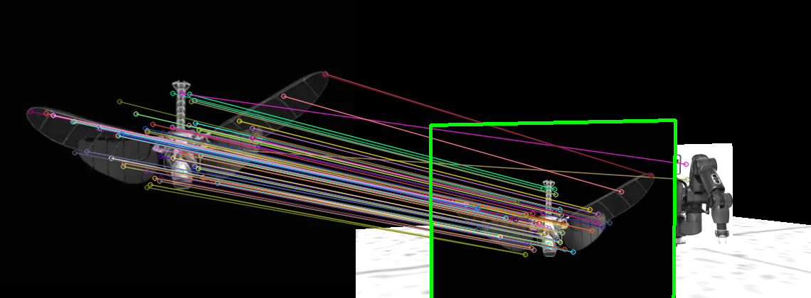
SURF would be applied to both the processed reference images and the world image separately. Their feature lists were then fed through the OpenCV searchInScene function to see how many features matched between the world and a given reference. If the portion of features that match across a pairing exceed a confidence threshold I set, it is considered a possible match.
Checking for features alone was not enough to be certain of what image was supposed to be caught, especially with multiple visible in a shot. To avoid this causing issues, an attempt is made to place a bounding box around any suspected match in the world’s image using homography. If the bounding box is self-intersecting (forms a bowtie shape) it is rejected as an invalid match. This check significantly reduced the number of false positives we encountered. If still valid but the area of this box is too small, the match is also rejected. If not, the area and feature match confidence are compared for a final match confidence for that reference (so closer boxes are preferred). This process is repeated for all possible tags.
Once all tags have be scanned for in the image, the top two final confidence are compared, if the highest one exceeds the second by some ratio, it is considered a proper match and is recorded for that box. If this ratio is not met or no confidence surpasses the minimum threshold, a blank is recorded instead of a specific tag.
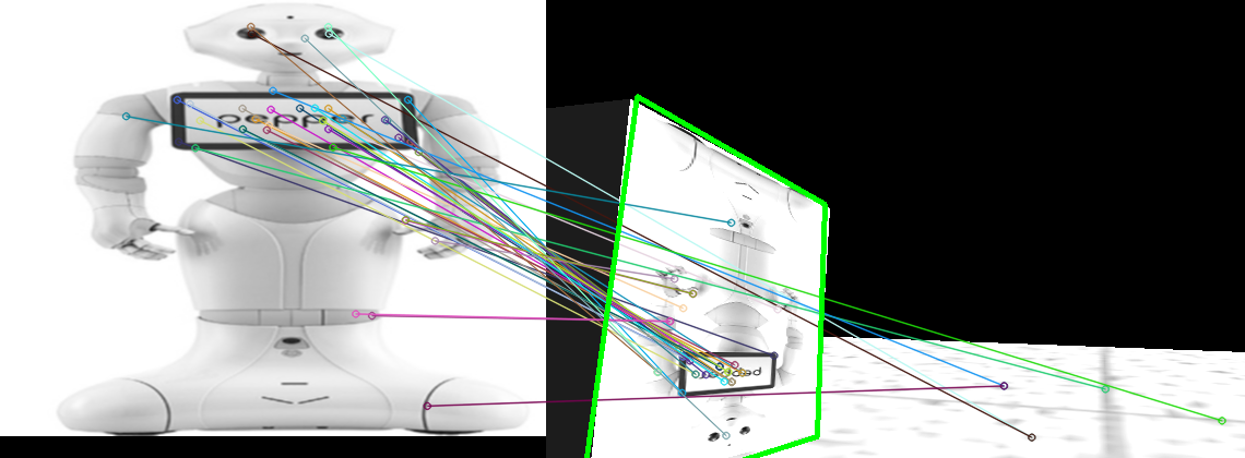
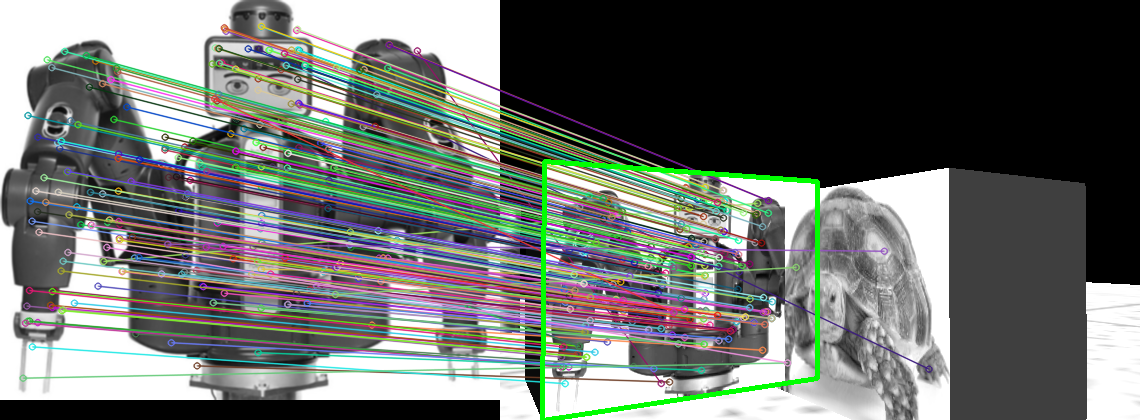
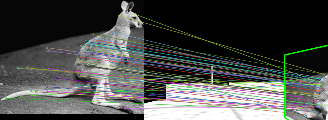
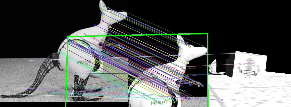
Testing Image Detection
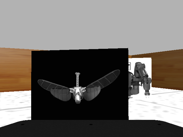
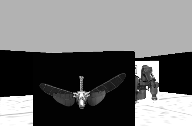
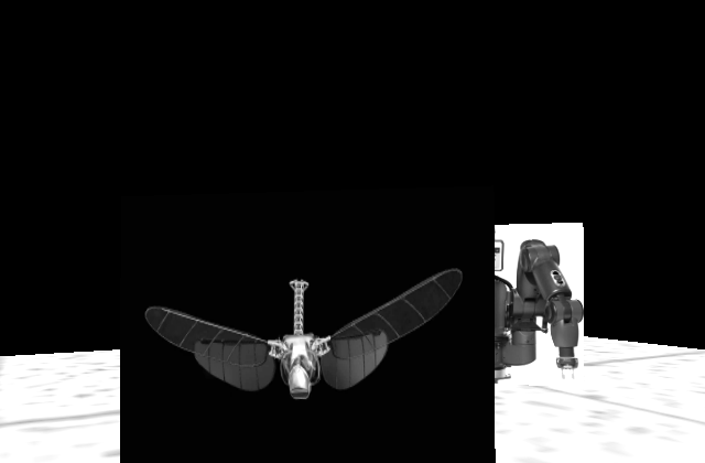
To test the image detection code in an efficient manner I collected a series of about 50 or 60 images taken from the simulator of various tags on different boxes with differing conditions, generally meant to be adverse to image recognition to properly exercise the system without needing to run the entire simulator every time. Below are some examples of the tests being passed.
Outputting Data
Output data was just a text file prepared that would be saved on the user’s computer listing the locations of boxes visited, the identified tag, and if it was the first time that tag was spotted (new) or if it was a duplicate (dup). These entries were ordered in the order the robot visited them. For example, if tag 2 was spotted for the first time on a box at (1.94 m, -1.41 m) with a orientation (heading) of 0.788 radians, the entry would be:
Tag 2 - ( 1.94, -1.41, 0.788) - new
Overall Structure
The overall structure of the code for milestone 2 was pretty basic. There was an initialization stage to start up all the ROS processes we need as well as determine the order of boxes to visit.
Then a loop was entered where the robot would go location to location as prescribed by the route, take an image, and see if there were a match present to record.
Once all stops were visited, the robot would return to its starting location as required, and exit the loop. It would then record its findings and terminate. The robot would also exit the loop if it hit the time limit. This wasn’t expected though since we were generally completing the runs in about four or so minutes of the eight allowed.
A full version of our code for this milestone is available at our contest 2 GitHub repository.
Contest 2 Results
Our code for these contest managed a perfect run! Our report also received a good review, you can read it here.
I even recorded a simulated run of this contest since I was so proud of it. I would recommend that you view it in 4K if possible to make out most of the details.
Copied from the description of the video:
An explanation of the windows going clockwise from the top left:
Top left (once program is running): Results of image scan using OpenCV. The left half of this window show the reference image spotted in the preprocessed scene on the right. The lines drawn between them are shared features.
Centre left: Live view of the raw video input the robot is provided.
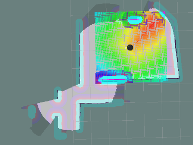
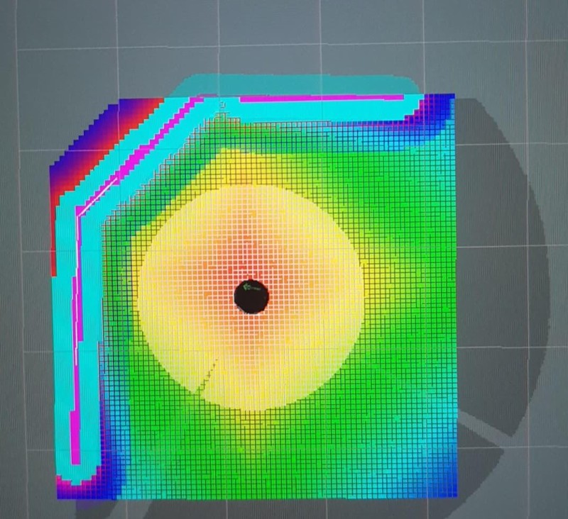
Centre right: Rviz localization and mapping visualization. Shows the location of the robot in the map provided (black obstacle outlines) and overlays it with the cost map (colour). The cost map is entirely based off of the proximity to an obstacle, thus urging the robot to avoid these regions when navigating. A planned path is drawn with a faith line between locations.
Top right: Gazebo simulation visualizer. Shows the state of the simulation the robot is operating in.
Bottom right: Console terminals. These are used to start each of the different processes needed to operate the robot and its simulation such as the mapping service and visualizers. The largest terminal window is where our code is executed and has its output displayed, such as the robot’s progress.
Left half / bottom left: VS Code IDE for developing the team’s code.
Milestone 3 - Search and Res-ponse?
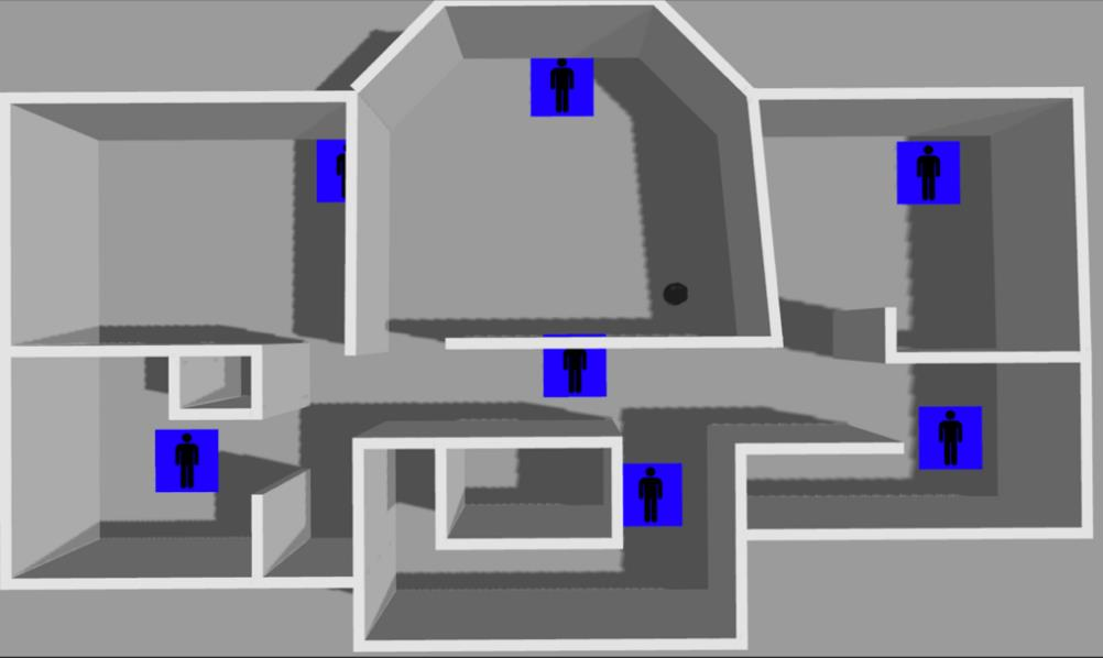
As the culmination of our previous efforts, this milestone required us to have the robot explore a “disaster” to find and provide instruction to the victims trapped within. This had the robot explore an unknown world for users to interact with (all we knew about the victims was that there were going to be seven present), and then interact appropriately given their emotional state as derived from their facial expression, for example trying to calm a distressed person while trying to provide instruction on how to exit the building.
The Disaster
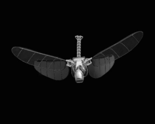
The exact disaster was up to each team to decide for themselves, the only requirement was that the interactions must be distinct and identifiable for each of the seven emotions we needed to identify. Our team chose the disaster to be a fight between Godzilla and King Kong, due to the recent movie that was released titled Godzilla vs. Kong (Adam Wingard, 2021). The victims are required to evacuate the building before Godzilla and King Kong begin to fight in the city, in the event that the building is demolished in the ensuing battle. The victims were required to get to the roof of the building as helicopters are helping to evacuate citizens.

To be completely honest I haven’t watched this movie yet, but it was a fun (impeding) disaster to work with anyway!
Exploration
To find the victims of the disaster, the robot would need to explore an enclosed, indoor space, segmented into multiple areas/rooms, on it’s own and in a timely manner.
Unlike in contest 1, we didn’t have to prepare the majority of the exploration algorithm. We instead primarily used the available Explore class in ROS to handle automated exploration. Simply calling Explore.start() and Explore.stop() were sufficient to run the exploration.
This exploration algorithm was built upon gmapping’s provided map of the world. We were used a “greedy” frontier-based exploration algorithm, where the robot takes the average location of all the frontiers (divisions between explored and unexplored areas, that are not obstacles) in its vicinity and heads to that average. This cycle is repeated again and again, even as the robot moves to make a constantly shifting target to reach.
The reason it is called “greedy” is because it is favouring the local optimum, not considering where the actual optimum exploration point is in the entire world that would likely reveal the most of the unexplored world.
We did not choose to change Explore in any way, since we found its behaviour suitable for what we were trying to do. We did however prepare some supporting code to intervene when Explore would get stuck. Due to its “greedy” algorithm, it would get stuck when it arrives at a frontier average that does not reveal enough of the map to determine a new local frontier average compared to the previous one. The robot would then stop moving since it believed there was no where else to go. To detect this condition, we had code to monitor the robot’s distance travelled in the last roughly 10 seconds, to see if the robot had not moved a reasonable amount (about a metre).
To “unstick” the robot there were two tricks we tried to use. The first was to have the robot complete a revolution where it was in the hopes new frontiers would be uncovered and move the local frontier centroid. If that failed, we would then clear the frontier “black list” in gmapping so the robot would then briefly consider the global frontier centroid briefly and move to it.
Emotion Detection
There were seven emotional states that our robot needed to identify for each victim: anger, disgust, fear, happiness, sadness, surprise, and neutral.
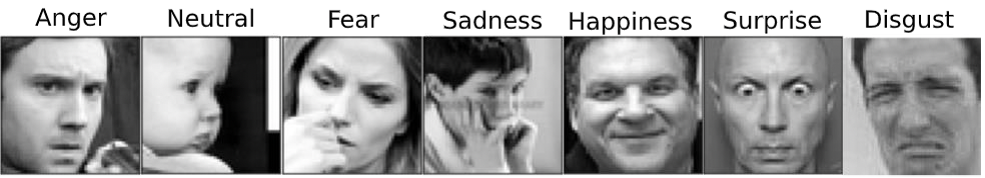
Emotion detection was to be achieved using a convolutional neural network (CNN) to classify the images of people’s faces.
The structure of the CNN can be split into two parts: the CNN and then a series of normal neural networks (NN). The images are first passed into the CNN which puts it through four stages of convolutions, which treat the pixels as a grid of numbers that have some effect on their neighbouring pixels. Once the four stages of convolutions are applied, the final NN takes the grid of values and combines them into just seven buckets (values), for the confidence that a given emotion is present in the given image.
A vital component of machine learning is training to fit the model to the data and this application was no exception. Ours was taught using “supervised” learning where the system is provided training data that has a corresponding set of expected outputs, e.g. an image of a child smiling in the training data would have a corresponding “happiness” entry in the expected output. These inputs are repeatedly fed in and compared to the needed outputs to try and tune the system iteratively to reduce amount of error in results.
For training the CNN we used a k-fold approach, where our training data was randomly and evenly split into k number of groups (folds). k models are trained using k-1 of the groups, and using the last group for validation. We used 5 folds, so 5 models were trained in parallel. Model one used folds 2 to 5 for training and then fold 1 for validation, model two would use fold 2 for validation and the others for training. This is used to make the most of our relatively limited test data set.
Once these five models were sufficiently trained, the one with the best performance on its validation set was selected and used in the final version of our code. The one we selected and used in our final project had achieved a success rate of almost 93%!
In the contest the robot would be provided eight separate images for a given victim, all showing the same emotion. So to determine the true emotion present, we would run each of the images through the model and combine their confidences to select the emotion with the highest combined confidence in the end.
Emotional Responses
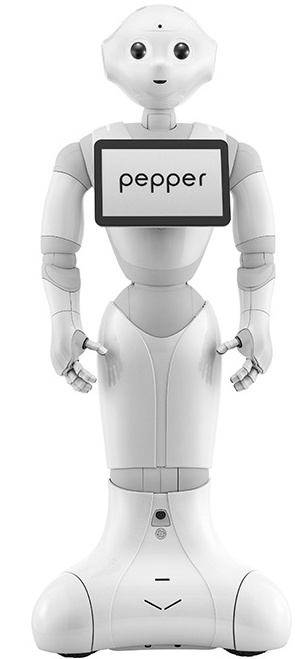
The emotional responses designed to be multi-modal (multiple degrees of expression) making use of the outputs available to us: the robot’s motions and the multimedia capabilities of the laptop (image and sound). In addition to making the robot more expressive by employing these additional outputs, it also helped us communicate with people with disabilities either permanent ones they have had or temporary as a result of the disaster (e.g. debris obscuring vision). Issuing commands with visuals and audio, as well as large motions for the visually impaired meant that at least one mode would be able to reach most people.
For each of the seven emotions victims would express, we had the robot express an emotion of its own in response, typically a different one to the victims. Here is a table of the emotions our would try to emulate when responding to a given emotion detected in the victim.
| Victim’s Emotion | Robot’s Response |
|---|---|
| Neutral | Pride |
| Happiness | Positively Excited |
| Fear | Embarrassment |
| Surprise | Surprise |
| Disgust | Discontent |
| Sadness | Anger |
| Anger | Resentment |
Each response was composed of between three to five steps that could be either a motion or media being played, but not both simultaneously. These are all laid out in Table 1 of our report. One of the responses, resentment, was enacted with the following sequence.
- Play sound of an unenthusiastic instruction to leave and show picture of or an emoji looking away
- Turn quickly 180 degrees
- Move straight short distance
- Turn back 100 degrees (as if to look over its shoulder)
- Play sound telling them that the robot is only trying to help them
We decided the overall emotion as a group, however my teammates worked on deciding the exact responses and generating the media needed. I transferred their ideas into code which was easy using the functions we had available:
- To perform the movements, the
travel()function was reused from Contest 1’s code. - To show images there was
showImage() - To play audio there was
soundPlayer.playWave()
Overall Structure
Just like in the first milestone, a finite state machine is used to regulate the robot’s behaviour by having it in a single state at a time with a defined procedure for changing between them. There were eight states: exploration and one for each of the seven emotional reactions. These states also had sub-states used to regulate finer aspects of each major state, for example, sub-states for emotional responses were used to progress through different the stages of the response.
The main behaviour of the robot was to explore until it came across a victim of the disaster at which point it would determine the emotion and switch to the appropriate reaction state. Once the reaction was completed, the rover would continue searching until all seven victims were found or the time limit was reached.
Once either of those end conditions were reached the robot would report reaching the condition and the time elapsed until then, cease exploring, and shutdown.
Contest 3 Results
We did well overall in this this trial. We were able to identify and react accordingly all emotions reliably, only failing in one of the 14 emotion checks we performed. However, there were some issues that caused the robot to spin in place for the entirety of the first trial (the TA manually moved the robot to test emotion recognition), although this was not repeated for the second trial where we managed to do everything with the exception of the one false identification.
Our report for contest three can be found here, it did well too.